While some feel GaN is still a relatively new technology, many can’t dispute how it’s advanced to the head of the class. AKA, Gallium Nitride, GaN is a technology on the cusp of dethroning silicon LDMOS, which has been the material of choice in high power applications. GaN is a direct bandgap semiconductor technology belonging to the III-V group. It is increasingly being used in power electronics because of its higher efficiency, superior high-voltage sustainability, reduced power consumption, higher temperature attributes, and power-handling characteristics.
These attributes have thrust GaN into the 5G RF spotlight – especially when it comes to mmWave 5G networks. And, while we all have ‘heard’ the promises of 5G, today, many of us in big cities – about 5 million of us to be more precise – are starting to realize those promises as major wireless carriers roll 5G out to their customers. But we are not there yet. Not even close. The goal is to connect 2.8 billion users by 2025. To reach this goal means to revamp the entire mobile infrastructure – a complex undertaking. But it can be done. And with the help of GaN technology, 5G will be in billions of people’s hands before you know it.
Recently, Embedded.com invited Qorvo’s own Roger Hall to pen a series of 5G articles that explain the complexities of building out the infrastructure and where GaN fits into the innovations that will bring 5G to the masses. Here are summaries of each article with a link for a deeper dive.
5G and GaN: Understanding Sub-6 GHz Massive MIMO Infrastructure
In this article, Roger explains the advantages for carriers to implement Massive MIMO technology as a means to minimize cost and increase capacity when rolling out 5G. He explores sub-6 GHz and why it’s important for increasing the adoption and expansion of 5G. He also addresses how GaN is being used in Massive MIMO Infrastructure applications. Read more >
5G and GaN: The Shift from LDMOS to GaN
Here Roger examines how the power demands of sub-6 GHz 5G base stations are driving a shift from silicon LDMOS amplifiers to GaN-based solutions, and what makes GaN a viable technology for many RF applications. Roger also reviews some of the tradeoffs engineers need to consider between these two technologies and why GaN is becoming the clear winner in many 5G solutions. Read more >
5G and GaN: What Embedded Designers Need to Know
Building on the previous article, Roger provides insight for embedded designers to fully realize the potential of GaN. He discusses misconceptions about GaN, explores its characteristics, and offers best practices to maximize its performance. Read more >
5G and GaN: Future Innovations
In his fourth and final article in this series, Roger looks to the future of GaN’s role in base stations. He provides a peek into GaN innovations being made today that will improve linear efficiency, power density and reliability and the implications of those improvements. Read more >
For more information on GaN technology, visit here.
About the Author
About Roger Hall
Roger is the General Manager of High-Performance Solutions at Qorvo. He leads program management and applications engineering for Wireless Infrastructure, Defense and Aerospace, and Power Management markets. This overarching role gives him a unique lens to view and interpret where RF technologies play fundamental parts in enabling future innovations.
Qorvo Blog Team
One part technical, one part content, and one part strategic, our small team is dedicated to connecting you with helpful, timely insights from some of the bright minds at Qorvo.
Original Blog link: https://www.qorvo.com/design-hub/blog/why-gan-is-5g-super-power
The AS8579 sensor offers the simplest way for car makers to comply with the UN Regulation 79, while giving the best detection performance
For automotive design engineers, it is unusual to find a new technology solution which performs better than existing approaches, and which reduces cost, and which is easier to implement in the application. But that is exactly what a new capacitive sensing chip, ams’ new AS8579, offers when used for hands-on detection (HOD) in cars which provide driver assistance functions.
It is the result of the application of a familiar and proven measurement principle – I/Q demodulation – to the job of sensing the position of the driver’s hands on the steering wheel. And it is markedly superior to any of the existing technologies in use for HOD in cars. Watch the highlights in our video:
Essential safety requirement in new car designs
The HOD function is required by the United Nations Regulation 79, and applies to all new cars that have a Lane Keeping Assist System (LKAS) wherever ratified. It has already been adopted by the European Union for new production vehicles from 1 April 2021. The purpose of the HOD system is to continuously monitor the readiness of the driver to assume control of the steering system in an emergency, or in the event of the failure of the LKAS.
Various technologies have been developed to provide this HOD function, but have had limitations: it is possible for drivers who want to avoid holding the steering wheel to fool the current monitoring system, which could compromise safety. And some existing solutions also perform poorly in certain operating conditions.
One approach to HOD has been the torque sensor: this detects the continual, minute deflections produced when the driver grips the steering wheel. The big drawback of this technology is that it can be easily fooled: the driver may take their hands off the wheel and ‘hold’ it by pressing upwards against it with their leg.
The problems with torque sensors have led the car industry to adopt a form of capacitive sensing for HOD: it monitors the driver’s grip on the steering wheel by detecting the change in capacitance of the steering wheel when the driver’s hands – which absorb electrical charge – come into contact with it. This technique only requires a single sensor chip connected to a metal sensor element built into the steering wheel.
Until now, automotive system manufacturers have used the charge-discharge method of capacitive sensing: this is a well understood technique, as it has been applied for many years in products such as touchscreens and touch-sensing buttons. But detection fails when the driver wears gloves, and false detection signals generated by the presence of moisture or humidity undermine the safety performance of hands-on detection based on this method of capacitive sensing. This type of capacitive sensor can even be fooled if the driver wedges a capacitive object, such as a piece of fruit or a plastic water bottle, into the frame of the steering wheel. So again, the implementation of this charge-discharge method of capacitive sensing potentially compromises safety.
It is true that other technologies are already applied to other driver-monitoring functions. For instance, 2D optical sensing is in use in systems for monitoring the position of the driver’s head. However, these 2D optical-sensing systems are not capable of performing HOD. This means that capacitive sensing is the most viable technology for HOD that is ready for deployment today. And now ams has a new approach to capacitive sensing which will meet all the safety requirements imposed by the automotive industry, and which is simple to implement.
Better performance, lower cost
This new solution from ams provides better performance, and with fewer components than the existing charge-discharge technique for capacitive sensing.
By implementing reliable capacitive sensing based on I/Q demodulation, the AS8579 capacitive sensor performs HOD in a way which cannot be fooled. Like the charge-discharge method, I/Q demodulation is a proven and well-known technique for capacitive sensing. Its advantage is that it measures the resistive as well as the capacitive element of a system’s impedance. The effect of this is that, unlike the charge-discharge method, it works reliably in difficult conditions, such as in the presence of moisture, or when the driver is wearing gloves. And it cannot be fooled, so provides for assured detection of the driver’s grip on the steering wheel. And the added benefit of the AS8579-based solution is that it can operate via a heated steering wheel’s heater element, so it does not require a separate sensor element to be built into the steering wheel.
This is how the AS8579 eliminates the normal trade-offs in engineering design:
It performs better – it cannot be fooled, and it operates in all conditions
It costs less – it is a single-chip solution, and requires no dedicated sensing element in a heated steering wheel
It is easy to implement – the chip’s output is an impedance measurement, and the system controller simply applies a threshold value to determine whether hands are on the steering wheel or not.
Ready for use in automotive designs
The AS8579 is fully automotive qualified, and offers multiple on-chip diagnostic functions, ensuring support for the ISO 26262 functional safety standard up to ASIL Grade B. Operating at one of four selectable driver-output frequencies – 45.45kHz, 71.43kHz, 100kHz or 125kHz – the AS8579 offers high immunity to electromagnetic interference.
Automotive designers can start developing with the AS8579 automotive capacitive sensor immediately using its dedicated evaluation kit, the AS8579-TS_EK_DB.
Andreas Zenz joined ams in 2013. Since then he has worked in application engineering for automotive, industrial, medical and robotics customers. In addition, he has taken on the product management role for the AS8579 automotive-qualified capacitive sensor.
Original blog post: https://ams.com/sensor-blog/1d-tof-family
ams 1D time-of-flight ranging sensor family offers mobile and industrial customers the right combination of performance, size, and cost to meet their needs.
When innovating sensor technology for a better lifestyle, ams engineers are balancing three attributes that are vital to customers: sensor performance, sensor size, and system cost. These variables are almost infinitely adjustable according to our customers’ evolving needs and specifications, competitive conditions, regulatory constraints or bill of materials requirements. How we design our product portfolio is based on our reading of the market and what our customers and close design partners tell us they want.
Customers are in a never-ending race to deliver better products and experiences. And as part of this, 1D Time-of-Flight sensors for front and world-facing applications are becoming increasingly important in the mobile, consumer, wearables, PC and industrial segments. The ams family of 1D ToF ranging sensors, developed for Laser Distance Auto-Focus (LDAF) applications within the mobile phone industry area also bringing benefit and increasingly winning in applications including PC user detection enabling auto lock/unlock, obstacle avoidance in robotic vacuum cleaners, inventory management, to name a few.
Broadening the family of time-of-flight (ToF) ranging sensors
ams has a strong history in bringing 1D ToF sensing innovations to market. Our most recent innovations include the world’s smallest 1D ToF sensor for accurate proximity sensing and distance measurement in smartphones’ – the TMF8701 and the TMF8801 which extends the operating range of the direct time of flight module to enable smartphones with space-saving accurate distance measurement. Now, ams brings rounds out the TMF sensor family with the TMF8805 adjusting the performance/cost variables to give customers greater flexibility and choice, especially for applications and products with massive growth potential or competing in the uncertainty of emerging markets.
TMF8805 – for mobile phone camera applications and more
The TMF8805 is a highly-integrated module which includes a class 1 eye-safe 940nm Vertical Cavity Surface Emitting Laser (VCSEL), Single Photon Avalanche Diode (SPAD) array, time-to-digital converter (TDC) along with a low power, high performance microcontroller. This system-in-module integration enables robust and precise distance measurements in the 20mm and 2500mm range, all packaged in the industry’s smallest footprint measuring only 2.2mm x 3.6mm x 1.0mm.
This high precision distance measurement is ideal for use in world-facing, LDAF mobile phone applications by enabling a fast, high-precision auto-focus feature. The new sensor joins the existing TMF8801 and TMF8701 time-of-flight sensors from ams, providing products which meet a range of cost and performance requirements across the mobile, wearable and consumer electronics, computing and industrial markets.
To meet evolving expectations in a transforming world, customers come to ams for our simple-to-integrate, plug-and-play sophisticated sensor systems, while often benefiting from the ‘speed premium’ of our supplier ecosystem and specialist expertise. The TMF8805 time-of-flight sensor is now in mass production and an evaluation kit featuring the TMF8805 along with a comprehensive evaluation GUI is also available.
Blog post from: https://www.knowles.com/about-knowles/blog/challenges-5g-brings-to-rf-filtering
In the race to implement mainstream 5G wireless communication, the world is waiting to see if this next-generation network will achieve a hundredfold increase in user data rates. This transformative technology not only boosts performance for the latest cell phones, but also for fixed wireless access (FWA) networks and Internet of Things (IoT) smart devices. In order to reach 10 Gbps peak data rates, the increase in channel capacity must come from somewhere. A key innovation at the heart of 5G is utilizing new frequencies greater than 20 GHz in the millimeter wave (mmWave) spectrum, which offers the most dramatic increase in available bandwidth.
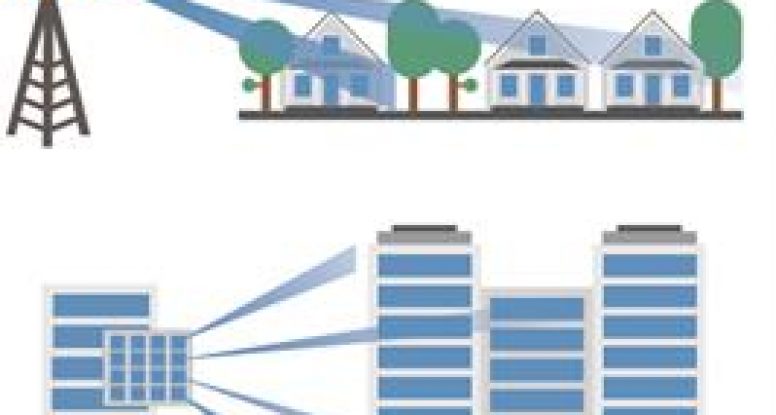
A well-known downside to high frequencies is the range limitation and path loss that occurs through air, objects, and buildings. The key workaround for mmWave base station systems is the use of multi-element beamforming antenna arrays in both urban and suburban environments. Since mmWave signals require much smaller antennas, they can be tightly packed together to create a single, narrowly focused beam for point-to-point communication with greater reach.
In order to overcome the range limitations of mmWave frequencies, dense arrays of antennas are used to create a tightly focused beam for point-to-point communication.
Changes in Radio Architecture for mmWave Beamforming
Of course, these new beamforming radio architectures bring a whole new set of challenges for designers. Traditional filtering solutions for radios operating in the ranges of 700 MHz and 2.6 GHz are no longer suitable for mmWave frequencies such as 28 GHz. For example, cavity filters are often used in the RF front ends of LTE macrocells. However, an inter-element spacing of less than half the wavelength (λ/2) is required to avoid the generation of grating lobes in antenna array systems. This inter-element spacing is about 21.4 cm at 700 MHz frequency versus only about 5 mm at 28 GHz. Such a requirement therefore calls for very small form factor components in the array. Not only will the whole RF front end be reduced in size, but also the number of RF paths will be increased – which means the filters right next to the antennas must be very compact.
As the frequency increases, the antenna size must decrease, leading to significant changes in the mmWave beamforming radio architecture.
Addressing Challenges with mmWave Filtering
Based on decades of experience working with mmWave filtering solutions, Knowles Precision Devices has a product line of mmWave filters solutions that addresses these challenges. Using specialized topologies and material formulations, we’ve created off-the-shelf catalog designs available up to 42 GHz that are 20 times smaller than the current alternatives.
Compared to current alternatives, Knowles Precision Devices offers filter solutions that are 20 times smaller to meet mmWave inter-element spacing requirements.
As manufacturers push to increase available bandwidth, temperature stability also becomes more and more of an issue. MmWave antenna arrays may be deployed in exposed environments with extreme temperatures, and heat dissipation issues may arise from packing miniature components onto densely populated boards. In order to guarantee consistent performance, our filters are rated for stable operation from -55°C to +125°C. For example, the bandpass filters below shifted only by 140 MHz when tested over that temperature range.
The temperature response of a Knowles 18 GHz band pass filter (BPF) on CF dielectric shows little variation in performance from -55°C to +125°C.
Finally, high performance with high repeatability is key to ensuring the best spectral efficiency and rejection possible. High frequency circuits are especially sensitive to variations in performance, so precise manufacturing techniques ensure that our filter specifications – such as 3 GHz bandwidth and greater than 50 dB rejection – are properly maintained from part to part. Plus, unlike chip and wire filter solutions, our surface mount filters standardize the form factor, reduce overall assembly time, and do not require tuning – thus saving in overall labor costs and lead times.
The performance of Knowles Precision Devices 37-40 GHz BPFs shows highly repeatable performance over 100 samples, even without post-assembly tuning.
As engineers, we’re always looking for the simplest solution to complex system design challenges. Look no further for solutions in the 5.2 GHz Wi-Fi realm. Here we step you through the resolutions to reduce design complexity, while meeting those tough final product compliance requirements.
An Essential Part of The Wi-Fi Tri-Band System
– 5.2 GHz RF Filters
Most individuals using Wi-Fi in any setting – home, office, or coffee shop – expect a fast upload and download experience. To achieve this, individuals and businesses must move toward a tri-band radio product solution. Anyone familiar with the two Wi-Fi bands of 2.4 GHz and 5 GHz, know the higher 5 GHz band is faster for upload and download speeds. However, the use of higher frequency bands comes at a price of signal attenuation. They also have a high probability of interference with other closely aligned spectrum.
This is where Qorvo filter technology comes in. Qorvo filters help mitigate these probable interferences. In this blog, we focus on the 5.2 GHz filter technology, the higher area of the Wi-Fi tri-band. This filter technology improves the mesh network quality-of-service and helps meet system regulatory requirements.
Wi-Fi and Cellular Frequency Bands
The 5 GHz band provides over six times more bandwidth than 2.4 GHz. This is a big plus for today’s video streaming, chatting, and gaming, which is in high demand. As shown in the figure below, spectrum re-farming and the crowding of wireless standards has increased. As Wi-Fi evolves into even higher realms of 5 GHz and 6 GHz, the crowding continues. As seen in the below figure, the 5 GHz unlicensed area clearly must coexist with cellular frequencies on all sides. One such area is the 5.2 GHz band.
Figure 1: Major wireless frequency bands for 5G Frequency Range (FR) 1 & 2
The Wi-Fi 5.2 GHz Space
The Wi-Fi 5 GHz UNII (Unlicensed National Information Infrastructure) arena is primarily used in routers in retail, service providers and enterprise spaces. These routers are commonly found in mesh networks, extenders, gateways and outdoor access points. In the UNII1-2a band (i.e. 5150-5350 MHz – 5.2 GHz band), maintaining a minimum RF system pathloss is important. Providing a minimum filter insertion loss is imperative to reduce power consumption, achieve better signal reception, and decrease thermal stress. This helps system designers to deliver low carbon footprint end-products. Additionally, for the 5.2 GHz band, a high out-of-band filter rejection is desired – notably around 50 dB or greater at 5490-5850 MHz – which helps mitigate crosstalk and enables coexistence with the 5.6 GHz UNII band, as shown in Figure 2 below.
To meet the need of the true mesh tri-band application, a well-designed filter is required. Today, few filter suppliers can meet the standard’s body specifications of rejection, insertion loss and power handling in the 5.2 GHz band. As shown in the below figure, Qorvo provides several filter solutions for the UNII 5 GHz bands.
Figure 2: 5 GHz UNII frequency bands, bandwidths, bandedge parameters, and filters
A Review of The Wi-Fi Standard Specifications
High Rejection – A high rejection is critical in a system for two main reasons – one being the need to mitigate interference, and two, to mitigate unwanted signal noise. Therefore, customers and standards bodies have set a desired high parameter of 50 dB or greater on rejection rate for critical out-of-band signals. But it is important to achieve this without losing the integrity of the RF signal range and capacity. Using Qorvo bandBoost™ filters such as the QPQ1903 achieves this goal.
As noted in Figure 2 above, coexistence with the Wi-Fi 5.6 GHz band has only a 120 MHz gap. Meeting the 50 dB or greater rejection at this frequency (5490-5850 MHz) within this small gap is challenging. It requires filter technologies with steep out-of-band skirts and a high rejection rate. BAW (bulk acoustic wave) SMR (solidly mounted resonator) technology is well suited to meet thermal and high rejection filter requirements. BAW-SMR has a vertical heat flux acoustic reflector that allows thermal heat to dissipate away quickly and efficiently from the filter. BAW exhibits very little frequency shifts due to self-heating as the topology of BAW-SMR provides a lower resistance, preventing the resonators from overheating. As shown in Figure 3 below, the rejection rate of the 120 MHz gap is greater than 50 dB, well within the regulatory guidance parameters.
Figure 3: 5.2 GHz QPQ1903 performance measurements @ 25⁰C Insertion Loss – In Figure 3 above, the insertion loss performance data for the 5.2 GHz bandBoost™ filter, QPQ1903, is 1.5 dB or better. Thus, providing improved system pathloss and power consumption. This translates directly to increased coverage range, better reception of the signal and simplified thermal management of the end product. Additionally, the return loss (not shown) meets the required specification by 2 dB or better across the entire pass band. This allows for an easier system match when using a discrete 5.2 GHz filter solution, which is especially critical in high linearity Wi-Fi 6 systems.
Power Handling – Power handling has become a major requirement for today’s wireless systems. 5G and the increases in RF input power levels to the receiver have attributed heavily to this new high-power handling system requirement. Thus, RF filters must be able to meet higher input power levels, sometimes up to 33 dBm. Luckily due to BAW-SMR’s ability to dissipate heat efficiently, it can easily attain this goal without compromising performance.
Not only has Qorvo BAW technology met the required critical regulatory specifications, but in most cases has done so with additional margin, and in the higher temperature ranges of up to 95⁰C – further helping customers and system designers meet stringent final product thermal management requirements.
New Wi-Fi System Complexity Challenges
The onset of Wi-Fi 6 and 6E standards has introduced additional application and system design complexity. Some of the most common challenges are:
Tri-band Wi-Fi
Smaller, sleeker device form factors
Higher temperature conditions due to form factor and application area requirements
Completely integrated solutions with no external tuning
Tri-band Wi-Fi – The need for data capacity and coverage has led to an explosion of the tri-band architecture of 2.4 GHz, 5.2 GHz and 5.6 GHz bands in gateways and end-nodes, as shown in Figure 4 below. It allows users to connect more devices to the internet using the 5 GHz spectrum in a more efficient way. For example, if you’re using a home mesh system with multiple routers to cover a larger space, the second 5.6 GHz band acts as a dedicated communications line between the two routers to speed up the entire system by as much as 180% over dual-band configurations.
Figure 4: 5.2 GHz & 5.6 GHz Wi-Fi filter response bandwidths and bandedge parameters Higher temperature conditions – New gateway designs require smaller form factors, sometimes half the size of previous product versions, with a higher number of RF antenna pathways (a tri-band router can have upwards of 8 RF pathways). Because of the confined space and increased number of antenna pathways, system thermal management becomes even more challenging. There are also gateway applications with higher temperatures at the extremes of -20⁰C to +95⁰C for outside environments.
Smaller form factor & integration – Today’s gateway devices are sleeker, stylish and have smaller form factors. The demand for smaller gateway form factors is pushing Wi-Fi integrated circuits to shrink as well. Additionally, this is moving semiconductor technologies toward creating smaller and thinner devices to mitigate system designer costs.
To accommodate this initiative, Qorvo has also integrated its filter technology into complete RF front-end designs to help system designers reduce design time, meet smaller size requirements, and increase time-to-market.
Figure 5: Comparison of 5 GHz ceramic versus Qorvo QPQ1903 BAW filters
As system designers continue to meet higher frequency demand initiatives – brought on by the hunger for more frequency spectrum – design challenges increase. New hurdles like system pathloss, signal attenuation, designs in higher frequency realms and meeting coexistence standards are becoming more prevalent. Qorvo has worked extensively with network standards bodies and customers across the globe to ensure their designs meet all compliance needs. We work hard to provide products that meet these highly sought-after specifications with additional margin. This proactive work ultimately allows our customers to concentrate on delivering best-in-class products rather than trying to mitigate difficult design and certification issues.
Have another topic that you would like Qorvo experts to cover? Email your suggestions to the Qorvo Blog team and it could be featured in an upcoming post. Please include your contact information in the body of the email.
About the Author
Qorvo Wi-Fi Experts
Four of our resident Wi-Fi product marketing, application, and R&D design experts, Mudar Aljoumayly, David Guo, Igor Lalicevic, and Jaidev Sharma, teamed up to create this blog post. Based on their collective knowledge of Wi-Fi device design, all have guided the advancement of filters for customers developing state-of-the-art Wi-Fi applications.
A Beginner’s Guide to Segmentation in Satellite Images: Walking through machine learning techniques for image segmentation and applying them to satellite imagery
Blog from: https://www.gsitechnology.com/
In my first blog, I walked through the process of acquiring and doing basic change analysis on satellite data. In this post, I’ll be discussing image segmentation techniques for satellite data and using a pre-trained neural network from the SpaceNet 6 challenge to test an implementation out myself.
What is image segmentation?
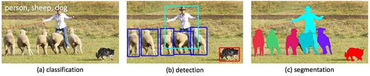
As opposed to image classification, in which an entire image is classified according to a label, image segmentation involves detecting and classifying individual objects within the image. Additionally, segmentation differs from object detection in that it works at the pixel level to determine the contours of objects within an image.
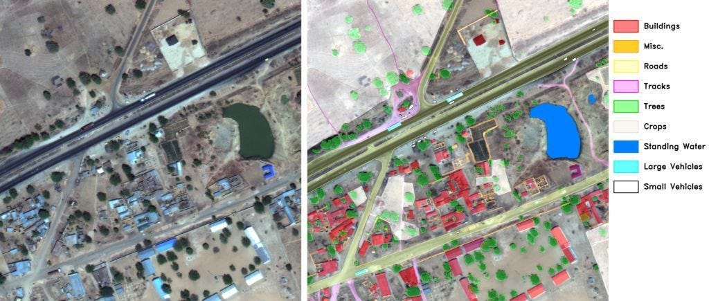
In the case of satellite imagery, these objects may be buildings, roads, cars, or trees, for example. Applications of this type of aerial imagery labeling are widespread, from analyzing traffic to monitoring environmental changes taking place due to global warming.
The SpaceNet project’s SpaceNet 6 challenge, which ran from March through May 2020, was centered on using machine learning techniques to extract building footprints from satellite images—a fairly straightforward problem statement for an image segmentation task. Given this, the challenge provides us with a good starting point from which we can begin to build understanding of what is an inherently advanced process.
I’ll be exploring approaches taken to the SpaceNet 6 challenge later in the post, but first, let’s explore a few of the fundamental building blocks of machine learning techniques for image segmentation to uncover how code can be used to detect objects in this way.
Convolutional Neural Networks (CNNs)
You’re likely familiar with CNNs and their association with computer vision tasks, particularly with image classification. Let’s take a look at how CNNs work for classification before getting into the more complex task of segmentation.
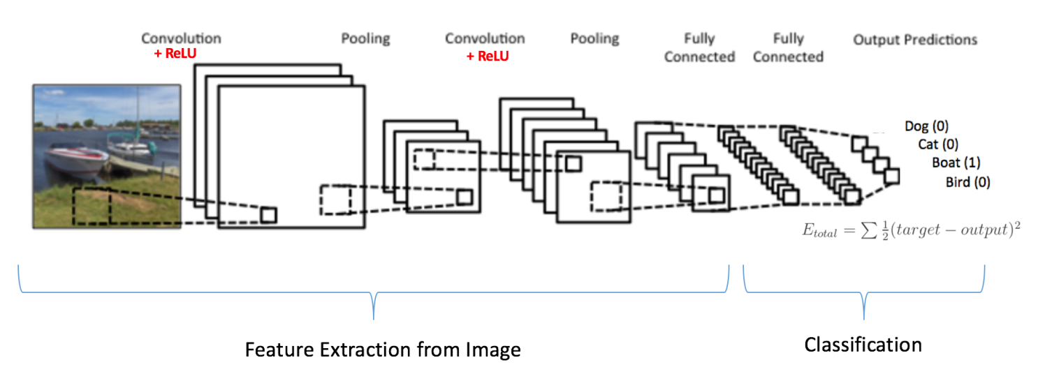
As you may know, CNNs work by sliding (i.e. convolving) rectangular “filters” over an image. Each filter has different weights and thus gets trained to recognize a particular feature of an image. The more filters a network has—or the deeper a network is—the more features it can extract from an image and thus the more complex patterns it can learn for the purpose of informing its final classification decision. However, given that each filter is represented by a set of weights to be learned, having lots of filters of the same size as the original input image makes training a model quite computationally expensive. It’s largely for this reason that filters typically decrease in size over the course of a network, while also increasing in number such that fine-grained features can be learned. Below is an example of what the architecture for an image classification task might look like:
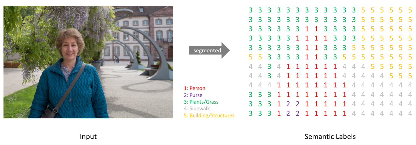
As we can see, the output of the network is a single prediction for a class label, but what would the output be for a segmentation task, in which an image may contain objects of multiple classes in different locations? Well, in such a case, we want our network to produce a pixel-wise map of classifications like the following:
An image and its corresponding simplified segmentation map of pixel class labels. Source
To generate this, our network has a one-hot-encoded output channel for each of the possible class labels:
These maps are then collapsed into one by taking the argmax at each pixel position.
The tricky part of achieving this segmentation is that the output has to be aligned with the input image—we can’t follow the exact same downsampling architecture that we use in a classification task to promote computational efficiency because the size and locality of the class areas must be preserved. The network also needs to be sufficiently deep to learn detailed enough representations of each of the classes such that it can distinguish between them. One of the most popular kinds of architecture for meeting these demands is what is known as a Fully Convolutional Network.
Fully Convolutional Networks (FCNs)
FCN’s get their name from the fact that they contain no fully-connected layers, that is, they are fully convolutional. This structure was first proposed by Long et al. in a 2014 paper, which I aim to summarize key points of here.
With standard CNNs, such as those used in image classification, the first layer of the network is fully-connected, meaning it has the same dimensions as the input image; this means that the size of the first layer must be fixed to align with the input image. Not only does this render the network inflexible to inputs of different sizes, it also means that the network uses global information (i.e. information from the entire image) to make its classification decision, which does not make sense in the context of image segmentation in which our goal is to assign different class labels to different regions of the image. Convolutional layers, on the other hand, are smaller than the input image so that they can slide over it—they operate on local input regions.
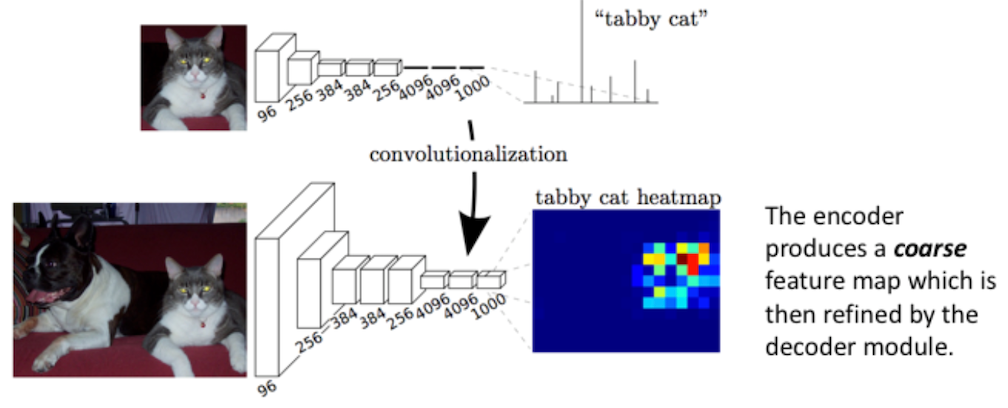
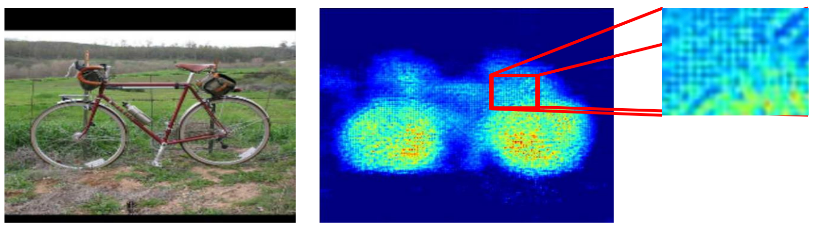
In short, FCNs replace the fully-connected layers of standard CNNs with convolutional layers with large receptive fields. The following figure illustrates this process. We see how a standard CNN for classification of a cat-only image can be transformed to output a heatmap for localizing the cat in the context of a larger image:
Moving through the network, we can see that the size of the layers getting smaller and smaller for the sake of learning finer features in a computationally efficient manner—a process known as “downsampling.” Additionally, we notice that the cat heatmap is of coarser resolution than the input image. Given these factors, how does the coarse feature map get translated back to the size of the input image at a high enough resolution such that the pixel classifications are meaningful? Long et al. used what is known as learned upsampling to expand the feature map back to the same size as the input image and a process they refer to as “skip layer fusion” to increase its resolution. Let’s take a closer look at these techniques.
Demystifying Learnable Upsampling
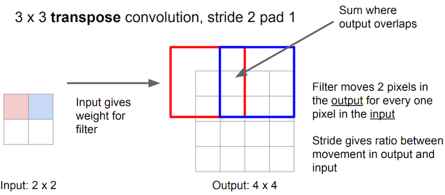
Prior approaches to upsampling relied on hard-coded interpolation methods, but Long et al. proposed a technique that uses transpose convolution to upsample small feature maps in a learnable way. Recall the way that normal convolution works:
The filter represented by the shaded area slides over the blue input feature map, computing dot products at each position to be recorded in the green output feature map. The weights of the filter are what is being learned by the network during training.
Transpose convolution works differently: the filter’s weights are all multiplied by the scalar value of the input pixel it is positioned over, and these values get projected to the output feature map. Where filter projections in the output map overlap, their values are added.
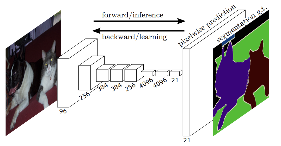
Long et al. use this technique to upsample the feature map rendered by network’s downsampling layers in order to translate its coarse output back to pixels that align with those of the input image, such that the network’s architecture looks like this:
An example of a final upsampling layer appended to the downsampling path to render a full-sized segmentation map. Note that the final feature map has 21 channels, representing the number of classes for the particular segmentation challenge being explored in the paper. Source
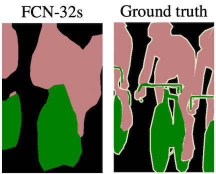
However, simply adding one of these transpose convolutional layers at the end of the downsampling layers yields spatially imprecise results, as the large stride required to make the output size match the input’s (32 pixels, in this case) limits the scale of detail the upsampling can achieve:
The upsampled segmentation map (left) is appropriately scaled to the input image but lacks spatial precision. Source
Luckily, this lack of spatial precision can be somewhat mitigated by “fusing” information from layers with different strides, as we’ll now discuss.
Skip Layer Fusion
As previously mentioned, a network must be deep enough to learn detailed features such that it can make faithful classification predictions; however, zeroing in closely on any one part of an image comes at the cost of losing spatial context of the image as a whole, making it harder to localize your classification decision in the process of zooming back out. This is the inherent tension at play in image segmentation tasks, and one that Long et al. work to resolve using skip connections.
In neural networks, a skip connection is a fusion between non-adjacent layers; in this case, skip connections are used to transfer local information by summing feature maps from the downsampling path with feature maps from the upsampling path. Intuitively, this makes sense: with each step we take through the downsampling path of the network, global information gets lost as we zoom into a particular area of the image and the feature maps get coarser, but once we have gone sufficiently deep to make an accurate prediction, we wish to zoom back and localize it, which we can do utilizing information stored in the higher resolution feature maps from the downsampling path of the network. Let’s take a more in depth look at this process by referencing the architecture Long et al. use in their paper:
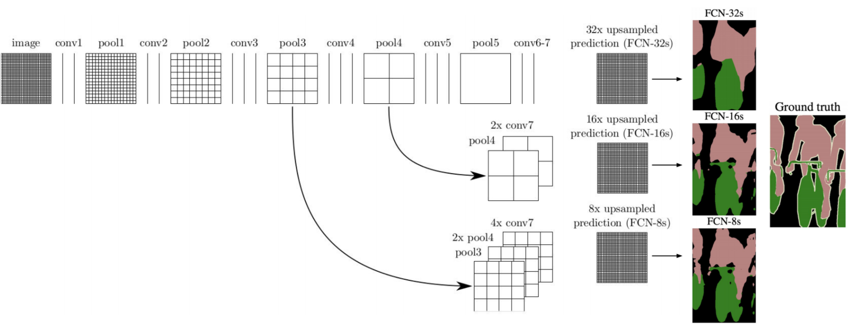
Visualization of skip connections (left arrows) in a network and their effect on the granularity of resulting segmentation maps. Source (modified)
Across the top of the image is the network’s downsampling path, which we can see follows a pattern of two or three convolutions followed by a pooling layer. conv7 represents the coarse feature map generated at the end of the downsampling path, akin to the cat heatmap we saw earlier. The “32x upsampled prediction” is the result of the first architecture without any skip connections, accomplishing all of the necessary upsampling with a single transpose convolutional layer of a 32 pixel stride.
Let’s walk through the “FCN-16s” architecture, which involves one skip connection (see the second row of the diagram). Though it is not visualized, a 1×1 convolution layer is added on top of the “pool4” feature map to produce class predictions for all its pixels. But the network does not end there—it proceeds to downsample by a factor of 2 once more to produce the “conv7” class prediction map. Since the conv7 map is of half the dimensionality of the pool4 map, it is upsampled by a factor of 2 and its predictions are added to those of the pool4, producing a combined prediction map. This result is upsampled via a transpose convolution with a stride of 16 to yield the final “FCN-16s” segmentation map, which we can see achieves better spatial resolution than the FCN-32s map. Thus, although the conv7 predictions experience the same amount of upsampling in the end as in the FCN-32s architecture (given that 2x upsampling followed by 16x upsampling = 32x upsampling), factoring the predictions from the pool4 layer improves the result greatly. This is because pool4 reintroduces valuable spatial information from the input image into the equation—information that otherwise gets lost in the additional downsampling operation for producing conv7. Looking at the diagram, we can see that the “FCN-8s” architecture follows a similar process, but this time a skip connection is also added from the “pool3” layer, which we see yields an even higher fidelity segmentation map.
FCNs—Where to go from here?
FCNs were a big step in semantic segmentation for their ability to factor in both deep, semantic information and fine, appearance information to make accurate predictions via an “encoding and decoding” approach. But the original architecture proposed by Long et al. still falls short of ideal. For one, it results in somewhat poor resolution at segmentation boundaries due to loss of information in the downsampling process. Additionally, overlapping outputs of the transpose convolution operation discussed earlier can cause undesirable checkerboard-like patterns in the segmentation map, which we see an example of below:
Criss-crossing patterns in a segmentation heatmap resulting from overlapping transpose convolution outputs. Source
Many models have built upon the promising baseline FCN architecture, seeking to iron out its shortcomings, “U-net” being a particularly notable iteration.
U-Net—An Optimized FCN
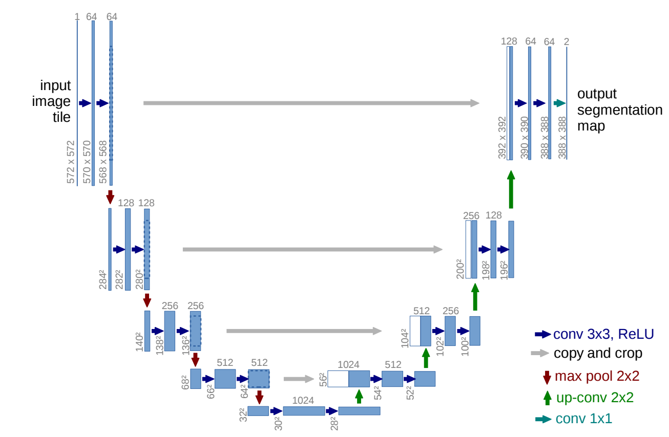
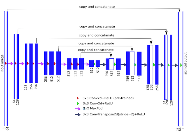
U-net was first proposed in a 2015 paper as an FCN model for use in biomedical image segmentation. As the paper’s abstract states, “The architecture consists of a contracting path to capture context and a symmetric expanding path that enables precise localization,” yielding a u-shaped architecture that looks like this:
An implementation of the U-net architecture. Numbers at the top of the feature maps denote their number of channels, numbers at the bottom left denote their x-y-size. The white feature maps represent are copies from the downsampling path, which we can see get concatenated to feature maps in the upsampling path. Source
We can see that the network involves 4 skip connections—after each transpose convolution (or “up-conv”) in the upsampling path, the resulting feature map gets concatenated with one from the downsampling path. Additionally, we see that the feature maps in the upsampling path have a larger number of channels than in the baseline FCN architecture for the purpose of passing more context information to higher resolution layers.
U-net also achieves better resolution at segmentation boundaries by pre-computing a pixel-wise weight map for each training instance. The function used to compute the map places higher weights on pixels along segmentation boundaries. These weights are then factored into the training loss function such that boundary pixels are given higher priority for being classified correctly.
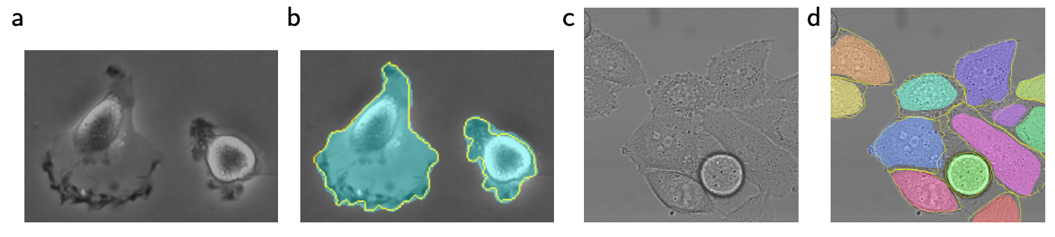
We can see that the original U-net architecture yields quite fine-grained results in its cellular segmentation tasks:
U-net segmentations results in images b and d, with ground truth boundaries outlined in yellow. Source
The development of U-net yet was another milestone in the field of computer vision, and five years later, models continue to expound upon its u-shaped architecture to achieve better and better results. U-net lends itself well to satellite imagery segmentation, which we will circle back to soon in the context of the SpaceNet 6 challenge.
Further Developments in Image Segmentation
We’ve now walked through an evolution of a few basic image segmentation concepts—of course, only scratching the surface of a topic at the center of a vast, rapidly evolving field of research. Here is a list of a few other interesting image segmentation concepts and applications, with links should you wish to explore them further:
Instance segmentation is a hybrid of object detection and image segmentation in which pixels are not only classified according to the class they belong to, but individual objects within these classes are also extracted, which is useful when it comes to counting objects, for example.
Techniques for image segmentation extend to video segmentation as well; for example, Google AI uses an “hourglass segmentation network architecture” inspired by U-net for real-time foreground-background separation in YouTube stories.
Clothing image segmentation has been used to help retailers match catalogue items with physical items in warehouses for more efficient inventory management.
Segmentation can be applied to 3D volumetric imagery as well, which is particular useful in medical applications; for example, research has been done on using it to monitor the development of brain lesions in stroke patients.
Many tools and packages have been developed to make image segmentation accessible to people of various skill levels. For instance, here is an example that uses Python’s PixelLib library to achieve 150-class segmentation with just 5 lines of code.
Now, let’s walk through actually implementing a segmentation network ourselves using satellite images and a pre-trained model from the SpaceNet 6 challenge.
The SpaceNet 6 Challenge
The task outlined by the SpaceNet challenge is to use computer vision to automatically extract building footprints from satellite images in the form of vector polygons (as opposed to pixel maps). In the challenge, predictions generated by a model are determined viable or not by calculating their intersection over union with ground truth footprints. The model’s f1 score over all the test images is calculated according to these determinations, serving as the metric for the competition.
The training dataset consists of a mix of mostly synthetic aperture radar (SAR) and a few electro-optical (EO) 0.5m resolution satellite images collected by Capella Space over Rotterdam, the Netherlands. The testing dataset contains only SAR images (for further explanation on SAR imagery, take a look at my last blog). The dataset being structured in this way makes the challenge particularly relevant to real-world applications, as SpaceNet explains, it is meant to “mimic real-world scenarios where historical optical data may be available, but concurrent optical collection with SAR is often not possible due to inconsistent orbits of the sensors, or cloud cover that will render the optical data unusable.”
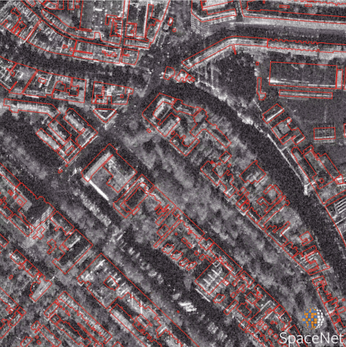
An example of a SAR image from the SpaceNet 6 dataset, with building footprint annotations shown in red. Source
More information on the dataset, including instructions for downloading it, can be found here. Additionally, SpaceNet released a baseline model, for which they provide explanation and code. Let’s explore the architecture of this model before implementing it to make predictions ourselves.
The architecture SpaceNet uses as its baseline is called TernausNet, a variant of U-Net with a VGG11 encoder. VGG is a family of CNNs, VGG11 being one with 11 layers. TernausNet uses a slightly modified version of VGG11 as its encoder (i.e. downsampling path). The network’s upsampling path mirrors its downsampling path, with 5 skip connections linking the two. TernausNet improves upon U-Net’s performance by initializing the network with weights that were pre-trained on Kaggle’s Carvana dataset. Using a model pre-trained on other data can reduce training time and overfitting—an approach known as transfer learning. In fact, SpaceNet’s baseline takes advantage of transfer learning again by first training on only the optical portion of the training dataset, then using the weights it finds through this process as the initial weights in its final training pass on the SAR data.
Even with these applications of transfer learning, though, training the model on roughly 24,000 images is still a very time intensive process. Luckily, SpaceNet provides the weights for the model at its highest scoring epoch, which allow us to get the model up and running fairly easily.
Making Predictions from the Baseline Model
Step-by-step instructions for deploying the baseline model can be found in this blog. In short, the process involves spinning up an AWS Elastic Cloud Compute (EC2) instance to gain access to GPUs for more timely computation and loading the challenge’s Amazon Machine Image (AMI), which is pre-loaded with the software, baseline model and dataset. Keep in mind that the dataset is very large, so downloads may take some time.
Once your downloads are complete, you can find the PyTorch code defining the baseline model in model.py. baseline.py takes care of image preprocessing and running training and testing operations. The weights of the pre-trained model with the best scoring epoch are found in the weights folder and are loaded when test.sh is run.
When we run an image through the model, it outputs a series of coordinates that define the boundaries of the building footprints we are looking to find as well as a mask on which these footprints are plotted. Let’s walk through the process of visualizing an image and its mask side-by-side to get a sense of how effective the baseline model is at extracting building footprints. Code for producing the following visualizations can be found here.
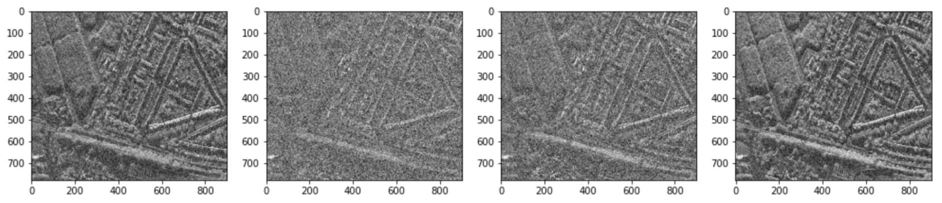
Getting a coherent visual representation of the SAR data is somewhat trickier than expected. This is because each pixel in a given image is assigned 4 values, corresponding to 4 polarizations of data in the X-band of the electromagnetic spectrum—HH, HV, VH and VV. In short, signals transmitted and received from a SAR sensor come in both horizontal and vertical polarization states, so each channel corresponds to a different combination of the transmitted and received signal types. These 4 channels don’t translate to the 3 RGB channels we expect for rendering a typical image. Here’s what it looks like when we select the channels one-by-one and visualize them in grayscale:
Visual representations of the 4 polarizations of a single SAR image. Image by author
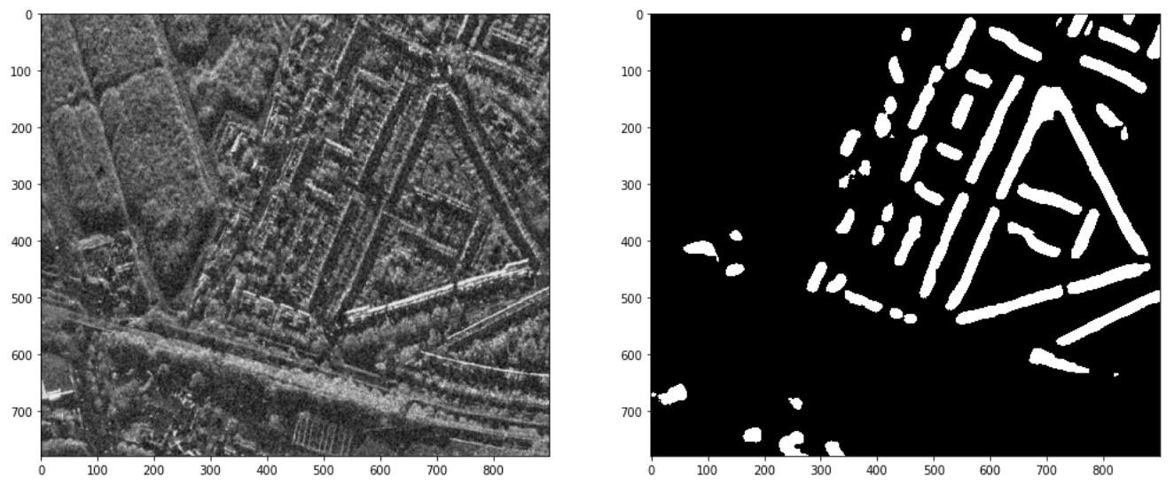
Notice that each of the 4 polarizations captures a slightly different representation of the same area of land. We can combine these representations to produce a single-channel span image to plot alongside the building footprint mask the model generated, which we convert to binary to make the boundaries more clear. With this, we can see that the baseline model did recognize the general shapes of several buildings:
A visualization of the combined spectral bands of a SAR test image and the corresponding building footprint mask generated by the baseline model. Image by author
It is pretty cool to see the basic structures we’ve discussed in this post in action here, producing viable image segmentation results. But, it’s also clear that there is room for improvement upon this baseline architecture—indeed, it only achieves an f1 score of 0.21 on the test set.
Conclusion
The SpaceNet 6 challenge wrapped up in May, with the winning submission achieving an f1 score of 0.42—double that of the baseline model. More details on the outcomes of the challenge can be found here. Notably, all of the top 5 submissions implemented some variant of U-Net, an architecture that we now have a decent understanding of. SpaceNet will be releasing these highest performing models on GitHub in the near future and I look forward to trying them out on time series data to do some exploration with change detection in a future post.
Lastly, I’m very thankful for the thorough and timely assistance I received from Capella Space for writing this—their insight into the intricacies of SAR data as well as recommendations and code for processing it were integral to this post.
The field of data science is rapidly changing as new and exciting software and hardware breakthroughs are made every single day. Given the rapidly changing landscape, it is important to take the appropriate time to understand and investigate some of the underlying technology that has shaped and will shape, the data science world. As an undergraduate data scientist, I often wish more time was spent understanding the tools at our disposal, and when they should appropriately be used. One prime example is the variety of options to choose from when picking an implementation of a Nearest-Neighbor algorithm; a type of algorithm prevalent in pattern recognition. Whilst there are a range of different types of Nearest-Neighbor algorithms I specifically want to focus on Approximate Nearest Neighbor (ANN) and the overwhelming variety of implementations available in python.
My first project with my internship at GSI Technology explored the idea of benchmarking ANN algorithms to help understand how the choice of implementation can change depending on the type and size of the dataset. This task proved challenging yet rewarding, as to thoroughly benchmark a range of ANN algorithms we would have to use a variety of datasets and a lot of computation. This would all prove to provide some valuable results (as you will see further down) in addition to a few insights and clues as to which implementations and implementation strategies might become industry standard in the future.
What Is ANN?
Before we continue its important to lay out the foundations of what ANN is and why is it used. New students to the data science field might already be familiar with ANN’s brother, kNN (k-Nearest Neighbors) as it is a standard entry point in many early machine learning classes.
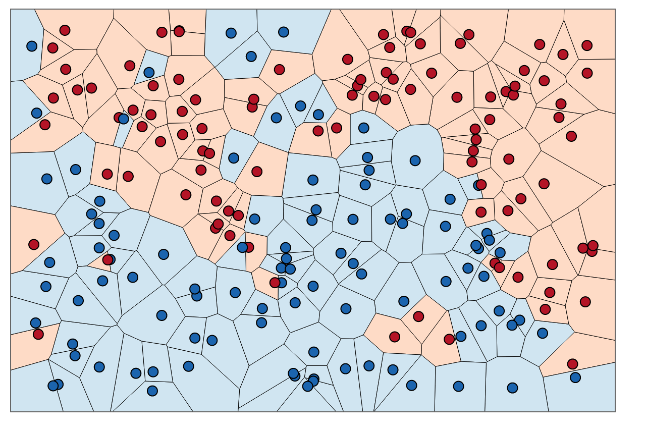
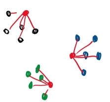
Red points are grouped with the five (K) closest points.
kNN works by classifying unclassified points based on “k” number of nearby points where distance is evaluated based on a range of different formulas such as Euclidean distance, Manhattan distance (Taxicab distance), Angular distance, and many more. ANN essentially functions as a faster classifier with a slight trade-off in accuracy, utilizing techniques such as locality sensitive hashing to better balance speed and precision. This trade-off becomes especially important with datasets in higher dimensions where algorithms like kNN can slow to a grueling pace.
Within the field of ANN algorithms, there are five different types of implementations with various advantages and disadvantages. For people unfamiliar with the field here is a quick crash course on each type of implementation:
Brute Force; whilst not technically an ANN algorithm it provides the most intuitive solution and a baseline to evaluate all other models. It calculates the distance between all points in the datasets before sorting to find the nearest neighbor for each point. Incredibly inefficient.
Hashing Based, sometimes referred to as LSH (locality sensitive hashing), involves a preprocessing stage where the data is filtered into a range of hash-tables in preparation for the querying process. Upon querying the algorithm iterates back over the hash-tables retrieving all points similarly hashed and then evaluates proximity to return a list of nearest neighbors.
Graph-Based, which also includes tree-based implementations, starts from a group of “seeds” (randomly picked points from the dataset) and generates a series of graphs before traversing the graphs using best-first search. Through using a visited vertex parameter from each neighbor the implementation is able to narrow down the “true” nearest neighbor.
Partition Based, similar to hashing, the implementation partitions the dataset into more and more identifiable subsets until eventually landing on the nearest neighbor.
Hybrid, as the name suggests, is some form of a combination of the above implementations.
Because of the limitations of kNN such as dataset size and dimensionality, algorithms such as ANN become vital to solving classification problems with these kinds of constraints. Examples of these problems include feature extraction in computer vision, machine learning, and many more. Because of the prominence of ANN, and the range of applications for the technique, it is important to gauge how different implementations of ANN compare under different conditions. This process is called “Benchmarking”. Much like a traditional experiment we keep all variables constant besides the ANN algorithms, then compare outcomes to evaluate the performance of each implementation. Furthermore, we can take this experiment and repeat it for a variety of datasets to help understand how these algorithms perform depending on the type and size of the input datasets. The results can often be valuable in helping developers and researchers decide which implementations are ideal for their conditions, it also clues the creators of the algorithms into possible directions for improvement.
Open Source to the Rescue
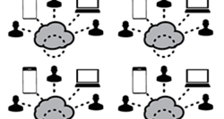
Utilizing the power of online collaboration we are able to pool many great ideas into effective solutions
Beginning the benchmarking task can seem daunting at first given the scope and variability of the task. Luckily for us, we are able to utilize work already done in the field of benchmarking ANN algorithms. Aumüller, Bernhardsson, and Faithfull’s paper ANN-Benchmarks: A Benchmarking Tool for Approximate Nearest Neighbor Algorithmsand corresponding GitHub repository provides an excellent starting point for the project.
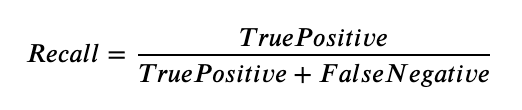
Bernhardsson, who built the code with help from Aumüller and Faithfull, designed a python framework that downloads a selection of datasets with varying dimensionality (25 to nearly 28,000 dimensions) and size (few hundred megabytes to a few gigabytes). Then, using some of the most common ANN algorithms from libraries such as scikit-learn or the Non-Metric Space Library, they evaluated the relationship between queries-per-second and accuracy. Specifically, the accuracy was a measure of “recall”, which measures the ratio of the number of result points that are true nearest neighbors to the number of true nearest neighbors, or formulaically:
Intuitively recall is simply the correct predictions made by the algorithm, over the total number of correct predictions it could have made. So a recall of “1” means that the algorithm was correct in its predictions 100% of the time.
Using the project, which is available for replication and modification, I went about setting up the benchmark experiment. Given the range of different ANN implementations to test (24 to be exact), there are many packages that will need to be installed as well as a substantial amount of time required to build the docker environments. Assuming everything installs and builds as intended the environment should be ready for testing.
Results
After three days of run time for the GloVe-25-angular dataset, we finally achieved presentable results. Three days of runtime was quite substantial for this primary dataset, however as we soon learned this process can be sped up considerably. The implementation of the benchmark experiment defaults to running benchmarks twice and averaging the results to better account for system interruptions or other anomalies that might impact the results. If this isn’t an issue, computation time could be halved by only performing the benchmark tests once each. In our case we wanted to match Bernhardsson’s results so we computed the benchmark with the default setting of two runs per algorithm which produced the following:
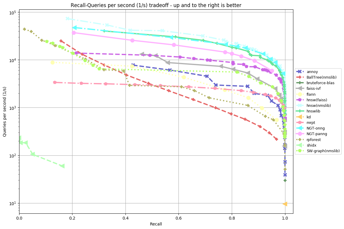
Our results (top) and Bernhardsson’s results (bottom):
My Results vs Bernhardsson’s Results
As you can see from the two side by side plots of algorithm accuracy vs algorithm query speed there are some differences between my results and Bernhardsson’s. In our case, there are 18 functions plotted as opposed to 15 in the other. This is likely because the project has since been updated to include more functions following Bernhardsson’s initial tests. Furthermore, the benchmarking was performed on a different machine to Bernhardsson’s which likely produced some additional variability.
What we do see which is quite impressive is that many of the same algorithms that performed well for Bernhardsson also performed well in our tests. This suggests that across multiple benchmarks there are some clearly well-performing ANN implementations. NTG-onng, hnsw(nmslib) and hnswlib all performed exceedingly well in both cases. Hnsw(nmslib) and hnswlib both belong to the Hierarchical Navigable Small World family, an example of a graph-based implementation for ANN. In fact, many of the algorithms tested, graph-based implementations seemed to perform the best. NTG-onng is also an example of a graph-based implementation for ANN search. This suggests that graph-based implementations of ANN algorithms for this type of dataset perform better than other competitors.
In contrast to the well-performing graph-based implementations, we can see BallTree(nmslib) and rpforest both of which in comparison are quite underwhelming. BallTree and rpforest are examples of tree-based ANN algorithms (a more rudimentary form of a graph-based algorithm). BallTree specifically is a hybrid tree-partition algorithm combining the two methods for the ANN process. It is likely a series of reasons that cause these two ANN algorithms to perform poorly when compared to HNSW or NTG-onng. However, the main reason seems to be that tree-based implementations execute slower under the conditions of this dataset.
Although graph-based implementations outperform other competitors it is worth noting that graph-based implementations suffer from a long preprocessing phase. This phase is required to construct the data structures necessary for the computation of the dataset. Hence using graph-based implementations might not be ideal under conditions where the preprocessing stage would have to be repeated.
One advantage our benchmark experiment had over Bernhardsson’s is our tests were run on a more powerful machine. Our machine (see appendix for full specifications) utilized the power of 2 Intel Xeon Gold 5115’s, an extra 32 GBs of DDR4 RAM totaling 64 GBs, and 960 GBs of solid-state disk storage which differs from Bernhardsson’s. This difference likely cut down on computation time considerably, allowing for faster benchmarking.
A higher resolution copy of my results can be found in the appendix.
Conclusion and Future Work
Further benchmarking for larger deep learning datasets would be a great next step.
Overall, my first experience with benchmarking ANN algorithms has been an insightful and appreciated learning opportunity. As we discussed above there are some clear advantages to using NTG-onng and hnsw(nmslib) on low dimensional smaller datasets such as the glove-25-angular dataset included with Erik Bernhardsson’s project. These findings, whilst coming at an immense computational cost, are none the less useful for data scientists aiming to tailor their use of ANN algorithms to the dataset they are utilizing.
Whilst the glove-25-angular dataset was a great place to start I would like to explore how these algorithms perform on even larger datasets such as the notorious deep1b (deep one billion) dataset which includes one billion 96 dimension points in its base set. Deep1b is an incredibly large file that would highlight some of the limitations as well as the advantages of various ANN implementations and how they trade-off between query speed and accuracy. Thanks to the hardware provided by GSI Technology this experiment will be the topic of our next blog.
Aumüller, Martin, Erik Bernhardsson, and Alexander Faithfull. “ANN-benchmarks: A benchmarking tool for approximate nearest neighbor algorithms.” International Conference on Similarity Search and Applications. Springer, Cham, 2017.
Liu, Ting, et al. “An investigation of practical approximate nearest neighbor algorithms.” Advances in neural information processing systems. 2005.
Malkov, Yury, et al. “Approximate nearest neighbor algorithm based on navigable small-world graphs.” Information Systems 45 (2014): 61–68.
Laarhoven, Thijs. “Graph-based time-space trade-offs for approximate near neighbors.” arXiv preprint arXiv:1712.03158 (2017).
LIDAR plays a major role in automotive, as vehicles perform tasks with less and less human supervision and intervention. As a leader in VCSEL, ams is helping to shape this revolution.
LIDAR (Light Detection and Ranging) is an optical sensing technology that measures the distance to other objects. It is currently known for many diverse applications in industrial, surveying, and aerospace, but is a true enabler for autonomous driving. As the automotive manufacturers continue their push to design and release high-complexity autonomous systems, we likewise develop the technology that will enable this. That is why ams continues to bring our high-power VCSELs to the automotive market and to test the limits on peak power, shorter pulses, and additional scanning features which enable our customers to improve their LIDAR systems.
In 2019, ams together with ZF and Ibeo announced a hybrid solution called True Solid State where, like flash technology, no moving parts are needed to capture the full scene around the vehicle. By sequentially powering a portion of the laser, a scanning pattern can be generated, combining the advantages of flash and scan systems.
Making sense of the LIDAR landscape
At ams, we classify LIDAR systems on seven elements: ranging principle, wavelength, beam steering principle, emitter technology and layout, and receiver technology and layout. Here we discuss the first five.
The most dominant implementation to measure distance (ranging) is Direct Time of Flight (DTOF): a short (few nanoseconds) laser pulse is emitted, reflected by an object and returned to a receiver. The time difference between sending and receiving can be converted into a distance measurement. Moreover, with duty cycles of <1% this system takes thousands of distance measurements per second. The laser pulse is typically in the 850-940nm rage, components are readily available and most affordable. However, systems can also be using 1300 or 1550nm, the big advantage is eye safety regulations allow more energy to be used here, and in theory, this provides more range. The downside is that components are expensive.
To scan the complete surroundings (or field of view) of a vehicle, the system needs to be able to shoot pulses in all directions. This is the beam steering principle. Classical systems used rotating sensor heads and mirrors to scan the field of view section by section. As these systems are bulky, they are being replaced by static systems with internal moving mirrors. MEMS mirrors are also about to enter the market. Another approach is flash, where no moving parts are needed at all. The light source illuminates the complete field of view, and the sensor captures that same field in a single frame like a photo. As the full scene is illuminated, and to remain eye safe, this means the range must be limited.
On the emitter side, edge emitters continue to be frequently used, based on earlier developments. They have a high-power density, making them suitable in combination with MEMS mirrors. Where first iterations were single emitters, meanwhile 2-4-8-16 emitters are being integrated in a single bar. Fiber lasers are another interesting technology. They offer even higher power density, and typically are used in 1550nm wavelength and come typically as a single emitter source.
ams is a leading supplier in the VCSEL emitter technology. Our high power VCSELs can differentiate in scan and flash applications as they are very stable over temperature, are less sensitive to individual emitter failures, and are easy to integrate. However, the best characteristic of VCSELs are their ability to form emitter arrays. This makes VCSELs easy to scale. It also allows for addressability, or powering selective zones of the die. This enables True Solid State topology, which we consider to be the most all-rounded LIDAR solution.
LIDAR enables Autonomous Driving
The most commonly accepted way to classify vehicles on their level of autonomy is by the definitions of the Society of Automotive Engineers (SAE). At SAE Level 3 and above, the vehicle takes over responsibility from the driver and assistance turns into autonomy. This means the vehicle should be able to perform its task without human supervision and intervention. This requires a step function in required system performance. Where Level 1 and Level 2 vehicles assist the driver and typically rely on camera or radar, or a combination, there are shortcomings in these technologies for 3D object detection. LIDAR technology addresses this, and there is wide consensus in the industry that from Level 3 onwards, LIDAR is needed for 3D object detection.
When 3D LIDAR is combined or fused with camera and radar, a high-resolution map of the vehicle’s surroundings can be constructed and allow the vehicle to safely fulfil its mission. The automotive industry started with more straightforward driver-assist use cases used in Level 1 and Level 2. As sensors and data processing gets more advanced, further more difficult use cases can be covered, such as Highway Pilot or City Pilot.
Ultimately, when every conceivable use case can be fulfilled by the system we define this as a Level 5 vehicle – fully autonomous and the holy grail of autonomous driving. This is expected to still be quite a number of years out from today. Moreover, there will be huge pressure to bring down cost and rationalize content per vehicle – to make autonomous driving available to the mass market.
Interested to learn more?
Let us know if you would like to discuss how you could be using ams technology to support your potential LIDAR applications! Contact ams sensor experts
5G is no longer just a promise—it’s very real, even though implementation is in its infancy. There are two examples from 2019 that demonstrate that 5G implementations are materializing. One is that Verizon launched 5G service in all its NFL football stadiums. The other example is that in South Korea, 5G subscribers reached more than 2 million by August of that year – just four months after local carriers commercially launched the technology. In this post, we explore what’s advancing 5G in these areas such as small cell densification, spectrum gathering, spectrum sharing and massive MIMO. Although it will take time to become ubiquitous, 5G is expected to be the fastest-growing mobile technology ever. According to the Global Mobile Supplier Association (GSA), 5G is expanding at a much faster pace than 4G LTE—approximately two years faster. GSA recently published data stating that more than 50 operators launched 5G mobile networks and at least 60 different 5G mobile devices are available across the world.
Ultimately, 5G will have a life-changing impact and transform many industries. However, for 2020, operators are focusing on supporting the first two major 5G use cases: faster mobile connectivity and fixed wireless access (FWA), which brings high-speed wireless connectivity.
The rapid pace of 5G development is highlighted in the 2nd edition of Qorvo’s 5G RF For Dummies book. This NEWLY UPDATED book describes key trends and technology enablers that are bringing 5G visions to life.
Here are some highlights in the book:
Network Densification and Small Cells
5G users will require more cell sites to greatly expand network capacity and support the increase in data traffic. This is prompting mobile network operators (MNOs) to rush and densify their networks using small cells—which are small, low-powered base stations installed on buildings, attached to lamp posts, and in dense city venues. These small cells will help MNOs satisfy the data-hungry users, improving quality-of-service.
Spectrum Gathering
5G requires vast amounts of bandwidth. More bandwidth enables operators to add capacity and increase data rates so users can download big files much faster and get jitter-free streaming in high resolution. The physical layer and higher layer designs are frequency agnostic, but separate radio performance requirements are specified for each. The lower frequency range (FR1), also called sub-7 GHz, runs from 410 to 7,125 MHz. The higher frequency range (FR2), also called millimeter Wave (mmWave), runs from 24.25 to 52.6 GHz.
5G RF For Dummies, Second Edition
Download and read this NEW UPDATED VERSION of our 5G RF For Dummies Book
To obtain the bandwidth in FR1 and FR2, more spectrum must be allocated. Already, regulators in roughly 40 countries have allocated new frequencies and enabled re-farming of LTE spectrum. However, much more will be needed. To provide at least some of that, 54 countries plan to allocate more spectrum between now and the end of 2022, according to the GSA.
4G to 5G Network Progression
5G Radio Access Network (RAN) is designed to work with existing 4G LTE networks. 3GPP allowed for multiple New Radio (NR) deployment options. Thus, making it easier for MNOs to migrate to 5G by way of a Non-Standalone (NSA) to Standalone (SA) option, as shown in the figure below.
Dynamic Spectrum Sharing
Dynamic spectrum sharing (DSS) is a new technology that can further help smooth the migration from 4G to 5G. With DSS, operators can allow 4G and 5G users to share the same spectrum, instead of having to dedicate each slice of spectrum to either 4G or 5G. This means operators can use their networks more efficiently and optimize the user experience by allocating capacity based on users’ needs. Thus, as the number of 5G users increases, the network can dynamically allocate more of the total capacity to each user.
Millimeter Wave (mmWave)
5G networks can deliver the highest data rates by using mmWave FR2 spectrum, where large expanses of bandwidth are available. mmWave is now a reality: 5G networks are using it for FWA and mobile devices and will apply it for other use cases in the future. Operators expect to roll out FWA to more homes, as 5G network deployment expands and suitable home equipment becomes available.
Massive MIMO
MIMO (multiple-input and multiple-output) increases data speeds and network capacity by employing multiple antennas to deliver several data streams using the same bandwidth. Many of today’s LTE base stations already use up to 8 antennas to transmit data, but 5G introduces massive MIMO, which uses 32 or 64 antennas and perhaps even more in the future. Massive MIMO is particularly important for mmWave because the multiple antennas focus the transmit and receive signals to increase data rates and compensate for the propagation losses at high frequencies. This brings huge improvements in throughput and energy efficiency.
RFFE Innovations that Enable 5G
Innovation in RF front-end (RFFE) technologies are needed to truly enable the vision of 5G. As handsets, base stations and other devices become sleeker and smaller, the RFFE will need to pack more performance into less space while becoming more energy-efficient. Some RF technologies are key in achieving these goals for 5G. They include:
Gallium Nitride (GaN). GaN is well suited for high-power transistors capable of operating at high temperatures. The potential of GaN PAs in 5G is only beginning to be realized. Their high RF power, low DC power consumption, small form factor, and high reliability enable equipment manufacturers to make base stations that are smaller and lighter in weight. By using GaN PAs, operators can achieve the high effective isotropic radiated power (EIRP) output specifications for mmWave transmissions with fewer antenna array elements and lower power consumption. This results in lighter-weight systems that are less expensive to install.
BAW Filters. The big increase in the number of bands and carrier aggregation (CA) combinations used for 5G, combined with the need to coexist with many other wireless standards, means that high-performance filters are essential to avoid interference. With their small footprint, excellent performance, and affordability, surface acoustic wave (SAW) and bulk acoustic wave (BAW) filters are the primary types of filters used in 5G mobile devices.
-Blog from https://www.qorvo.com/
Author – David Schnaufer
Technical Marketing Communications Manager
David is the public voice for Qorvo’s applications engineers. He provides technical insight into RF trends as well as tips that help RF engineers solve complex design problems.
Premstaetten, Austria (09 January, 2019) — ams (SIX: AMS), a leading worldwide supplier of high performance sensor solutions, today launched a miniature spectral sensor chip that brings laboratory-grade multi-channel color analysis capability to portable and mobile devices.
In end products such as mobile phones or accessories, the new AS7341 from ams produces more precise spectral measurements in a wider range of lighting conditions than competing sensors. The new sensor’s small dimensions also mean that it is easier to accommodate it in mobile phones and other portable devices.
“The AS7341 marks a breakthrough in the category of spectral sensors in a small package suitable for mounting in a mobile phone or consumer device. It is the smallest such device to offer 11 measurement channels, and also offers higher light sensitivity than any other multi-channel spectral sensor aimed at the consumer market,” says Kevin Jensen, Senior Marketing Manager in the Optical Sensors business line at ams.
Consumer benefits of the AS7341 include improved performance in mobile phone cameras, as the chip’s accurate spectral measurements enable superior automatic white balancing, more reliable light source identification and integrated flicker detection. The technology will more accurately reproduce colors and minimize distortion of ambient light sources, resulting in sharper, clearer and more true-to-color photographs. The AS7341 also will enable consumers to use their mobile devices to match the colors of objects such as fabrics through using color references like the PANTONE® Color System.
The power of the AS7341 to upgrade color measurement performance is demonstrated by the introduction of the Spectro 1™ portable colorimeter from Variable (www.variableinc.com). In the Spectro 1, Variable has used the AS7341 to provide professional color measurement for solid colors at a consumer price point. The product provides highly repeatable spectral curve data in 10nm increments across the visible light spectrum from 400nm to 700nm – a capability previously only available in professional spectrophotometers costing more than ten times as much as the portable Spectro 1.
“In our opinion, no other spectral sensor IC comes close to offering the multi-channel capability of the AS7341 from ams in such a compact chip package,” says George Yu, CEO of Variable. “This small size is a crucial benefit – integration with a mobile phone app is one of the key features of Spectro 1, and we have designed the product to be small enough to hold easily in one hand. And the multi-channel spectral measurements provided by the AS7341 mean that users of Spectro 1 will never be misled by false matching of metameric pairs.”
The AS7341 is a complete spectral sensing system housed in a tiny 3.1mm x 2.0mm x 1.0mm LGA package with aperture. It is an 11-channel device which provides extremely accurate and precise characterizations of the spectral content of a directly measured light source, or of a reflective surface. Eight of the channels cover eight equally spaced portions of the visible light spectrum. The device also features a near infrared channel, a clear channel, and a channel dedicated to the detection of typical ambient light flicker at a frequency of 50Hz upto 1kHz.
Beside camera image optimization, the AS7341 spectral sensor also supports various applications, such general color measurement of materials or fluids, skin tone measurement, and others.
The AS7341, which will be demonstrated at CES 2019 (Las Vegas, NV, 8-11 January 2019) is available for sampling. Mass production starting in February. Unit pricing is $2.00 in an order quantity of 10,000 units.
An evaluation board for the AS7341 spectral sensor is available. For sample requests or for more technical information, please go to >> ams.com/AS7341.