Blog post from Knowles Precision Devices. Starvoy represents Knowles Precision Devices across Canada, for further information on their range of highly engineered Capacitors and Microwave to Millimeter Wave components for use in critical applications in military, medical, electric vehicle, and 5G market segments.
To protect people and critical equipment, military-grade electronic devices must be designed to function reliably while operating in incredibly harsh environments. Therefore, instead of continuing to use traditional silicon semiconductors, in recent years, electronic device designers have started to use wide band-gap (WBG) materials such as silicon carbide (SiC) to develop the semiconductors required for military device power supplies. In general, WBG materials can operate at much higher voltages, have better thermal characteristics, and can perform switching at much higher frequencies. Therefore, SiC-based semiconductors provide superior performance compared to silicon, including higher power efficiency, higher switching frequency, and higher temperature resistance as shown in Figure 1.
.webp?width=1200&height=627&name=SiC-Based%20Semiconductors%20(1).webp)
As the shift to using SiC-based semiconductors continues, other board-level components, such as capacitors, must change as well. For example, as systems operate at higher frequencies, the capacitance needed decreases, leading to many instances where film capacitors can be replaced by ceramic capacitors.
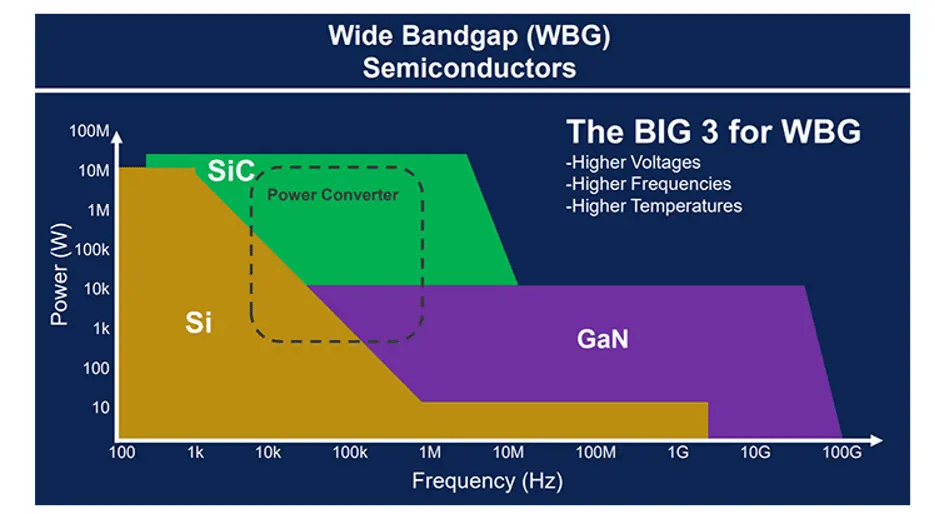
Figure 1. A comparison of traditional silicon semiconductor material to WBG materials such as SiC and GaN. Source.
Why You Need to Use Ceramic Capacitors with Your SiC Semiconductors
In general, ceramic capacitors are small and lightweight, making ceramic capacitors an ideal option for military applications where space and weight are at a premium. When using SiC semiconductors specifically, since the switching speeds are quite fast, high-frequency noise and voltage spikes will occur. Ceramic capacitors are needed to filter out this noise. And for high-frequency power supplies applications, ceramic capacitors are a preferred option because these components have a high self-resonant frequency, low equivalent series resistance (ESR), and high thermal stability.
Knowles Precision Devices: Your Military-Grade Ceramic Capacitor Experts
As a manufacturer of specialty ceramic capacitors, Knowles provide a variety of high-performance, high-reliability capacitors that are well-suited for military applications. At a basic level, they build all of their catalog and custom passive components to MIL-STD-883, a standard that “establishes uniform methods, controls, and procedures for testing microelectronic devices suitable for use within military and aerospace electronic systems.” We also hold the internationally recognized qualification for surface mount ceramic capacitors tested in accordance with the requirements of IECQ-CECC QC32100 as well as a variety of other quality certificates and approvals. For their high-reliability capacitors, they go above and beyond these quality standards and ensure components are burned-in at elevated voltage and temperature levels and are 100 percent electrically inspected to conform to strict performance criteria
Please contact the Starvoy team for further information, or to discuss your requirements.
Blog post from Knowles Precision Devices. Starvoy represents Knowles across Canada, for further information please reach out to our sales team.
As electric vehicle (EV) adoption for both consumer and commercial purposes rapidly grows, so does the need for a more widespread, and faster, charging infrastructure. While we’ve seen vast improvements in charging technology in the last few years, as additional regulations on combustion vehicles are implemented and reliance on EVs increases, further EV charging innovations are needed. Currently, wireless charging is the newest EV charging technology evolving.
Read More›In this industry, it can be easy to take power for granted. Easy, of course, until you don’t have it. Managing that vital resource is critical for systems to operate properly, and in a world that demands smaller, faster and smarter devices, it can be a real challenge. But what if a built-in power management device helped tackle that job? Qorvo’s Configurable Intelligent Power Solutions (ActiveCiPS™) devices help control, monitor and optimize power distribution and conversion in different systems with built-in intelligence and configurability.
In complex systems, or when a designer needs a more advanced or innovative power solution, it can be too expensive to use discrete components. Power Management Integrated Circuits (PMICs) integrate multiple voltage regulators and control circuits into a single chip. Today’s PMICs are flexible, allowing users to update default settings like output voltages, sequencing, fault thresholds and other parameters. As a result, PMICs are used in many small devices such as wearables, hearables and IoT (Internet of Things) devices – all thanks to their small size, high efficiency and low power consumption. These tiny, high-performance PMICs maximize system efficiency and performance while providing design flexibility and lowering the bill-of-materials cost.
Read More›
Original post from: https://www.qorvo.com/design-hub/blog/what-designers-need-to-know-to-achieve-wi-fi-tri-band-gigabit-speeds-and-high-throughput
Engineers are always looking for the simplest solution to complex system design challenges. Look no further for answers in the U-NII 1-8, 5 and 6 GHz realm. Here we review how state-of-the-art bandBoost™ filters help increase system design capacity and throughput, offering engineers an easy, flexible solution to their complex designs, while at the same time helping to meet those tough final product compliance requirements.
A Summary of Where We are Today in Wi-Fi
Wi-Fi usage has grown exponentially over the years. Most recently, it has skyrocketed upward to unimaginable levels — driven by the pandemic of 2020 due to work from home, school requirements, gaming advancements, and, of course, 5G. According to Statista, the first weeks of March 2020 saw an 18 percent increase in in-home data usage compared to the same period in 2019, with average daily data usage rates exceeding 16.6 GB.
With this increase in usage comes an increase in expectations to access Wi-Fi anywhere — throughout the home, both inside and out, and at work. Meeting these expectations requires more wireless backhaul equipment to transport data between the internet and subnetworks. It also requires advancements in existing technology to reach the capacity, range, signal reliability and the rising number of new applications wireless service providers are seeing. Figure 1 shows the exponential increase in wireless applications — from email to videoconferencing, smart home capabilities, gaming and virtual reality — as wireless technology continues to advance.
Go In Depth:
- Read Qorvo’s white paper that provides a play-by-play of how Wi-Fi has evolved over the past 20 years.
- Learn more about our industry-leading BAW Filter solutions.
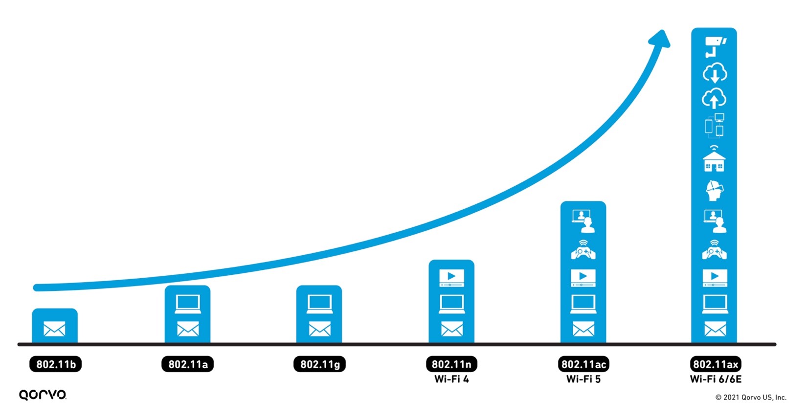
Figure 1: The advancement of Wi-Fi
The 802.11 standard has now advanced onto Wi-Fi 6 and Wi-Fi 6E, providing service beyond 5 GHz and into the 6 GHz area up to 7125 GHz, as shown in Figure 2. This higher frequency range increases our video capacities for our security systems and streaming.
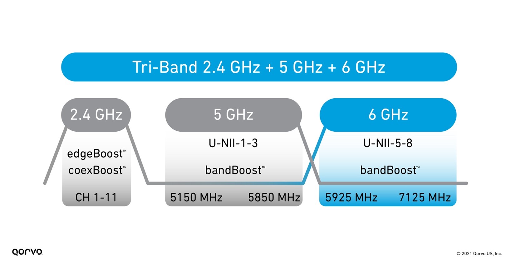
Figure 2: Tri-Band Wi-Fi frequency bands
However, working in higher frequency ranges can bring challenges such as more signal attenuation and thermal increases — especially when trying to meet the requirements of small form factors. To meet these challenges head-on, RF front-end (RFFE) engineers need to take existing technology to another level. One of those advancements has been in BAW filter technology now being used heavily in Wi-Fi system designs.
As shown in Figure 3 below, Qorvo has three BAW filter variants that boost overall Wi-Fi performance, maximize network capacity, increase RF range, and mitigate interference between the many different in-home radios operating simultaneously.
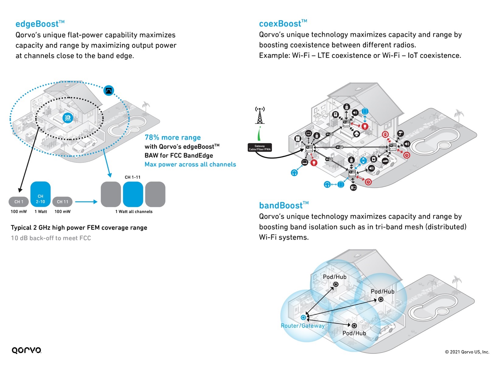
Figure 3: bandBoost, edgeBoost, and coexBoost filter technology performance
5 & 6 GHz bandBoost Filters
In a previous blog post called An Essential Part of The Wi-Fi Tri-Band System – 5.2 GHz RF Filters, we explored how using bandBoost filters like the Qorvo QPQ1903 and QPQ1904 can help reduce design complexity and help with coexistence. We also explored how these bandBoost filters provide high isolation, helping to reduce that function on the antenna design, allowing for less expensive antennas. Therefore, the RFFE isolation parameter no longer needs to rest entirely on the antenna. This reduces antenna and shielding costs – providing up to a 20 percent cost reduction.
These bandBoost BAW filters play a key role in separating the U-NII-2A band from the U-NII-2C band, which only has a bandgap of 120 MHz, as shown in Figure 4. Using these filters, we can attain Wi-Fi coverage reaching every corner of the home with the highest throughput and capacity. Using this solution in a Wi-Fi system design has shown increases in capacity for the end user up to 4-times.
Unlicensed National Information Infrastructure (U-NII)
The U-NII radio band, as defined by the United States Federal Communications Commission, is part of the radio frequency spectrum used by WLAN devices and by many wireless ISPs.
As of March 2021, U-NII consists of eight ranges. U-NII 1 through 4 are for 5 GHz WLAN (802.11a and newer), and 5 through 8 are for 6 GHz WLAN (802.11ax) use. U-NII 2 is further divided into three subsections: A, B and C.
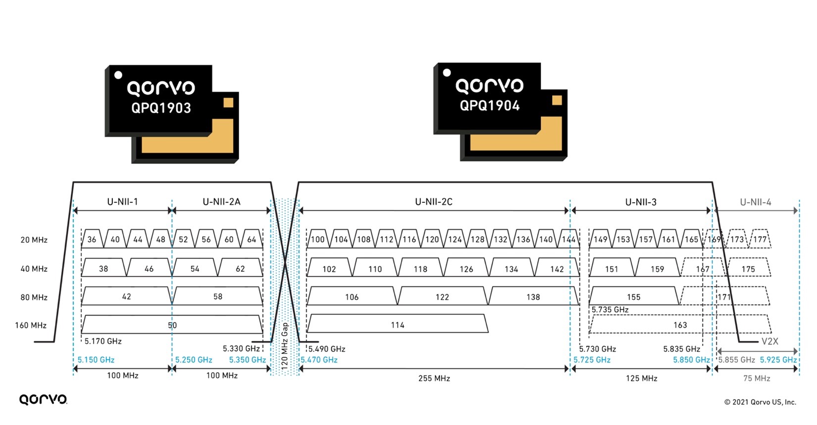
Figure 4: 5 GHz bandBoost filters and U-NII 1-4 bands
These filters are much smaller than legacy filters on the market used in Wi-Fi applications — allowing for more compact tri-band radios. They also have superior isolation achieving greater than 80 dBm system isolation for designers. This helps engineers meet the stringent Wi-Fi 6 and 6E requirements.
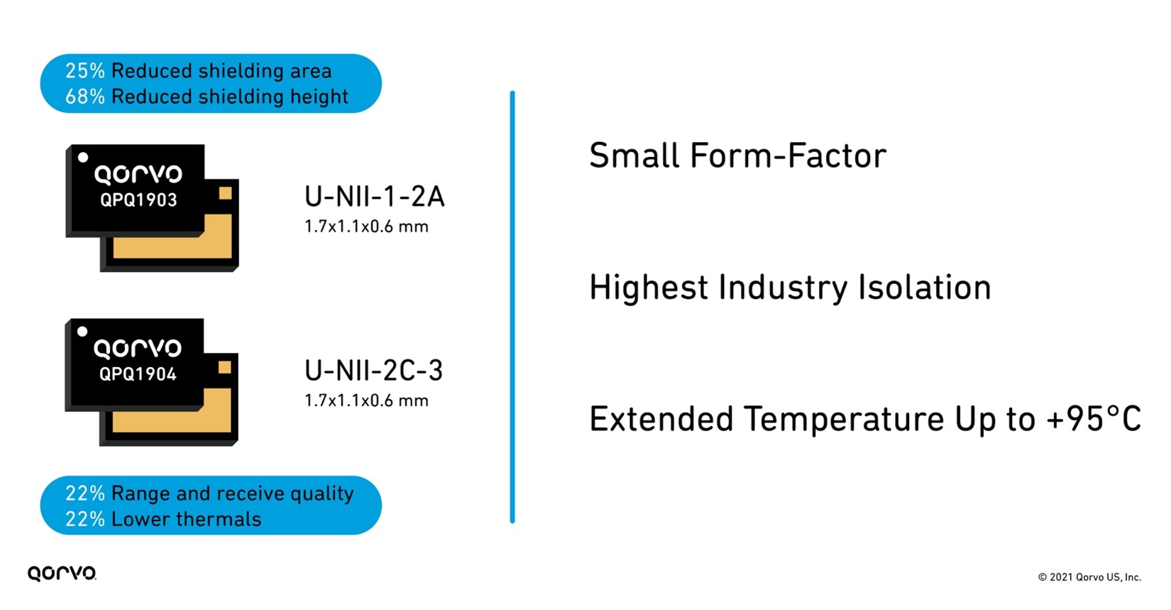
Figure 5: Benefits of using QPQ1903 and QPQ1904 bandBoost filters
The addition of multiple-input multiple-output (MIMO) and higher frequencies in the 6 GHz range increases system temperatures. With more thermal requirements, robust RFFE components are a must. Much of the industry specifies their parts in the 60°C to 80°C range, but higher temperature operation is needed based on the system temperatures produced in this frequency range. To solve these challenges, many hours of design effort have been spent on increasing the temperature capabilities of BAW. As product designs in Wi-Fi 5, 6/6E, and soon to come Wi-Fi 7, development has become more challenging, and as new opportunities like the automotive area opened for BAW, the push for higher temperature capability has come to the forefront.
Qorvo BAW technology engineers have delivered innovative devices by designing those that exceed the usual 85°C maximum temperature working range, going up to +95°C. The benefits this creates are great for both product designers and end-product customers. Now sleeker devices are achievable, as end-products no longer require large heat sinks. This also reduces design time as engineers can more easily attain system thermal requirements. One other advancement related to heat is that the bandBoost BAW products work at +95°C while still meeting a 0.5 to 1 dBm insertion loss.
This lower insertion loss improves Wi-Fi range and receive quality by up to 22 percent. Lower insertion loss also means improved thermal capability and performance as the RF signal seen at the RFFE Low Noise Amplifier (LNA) is improved. Below, Figure 6 shows the features and benefits of the QPQ1903 and QPQ1904 edgeBoost™ BAW filter.
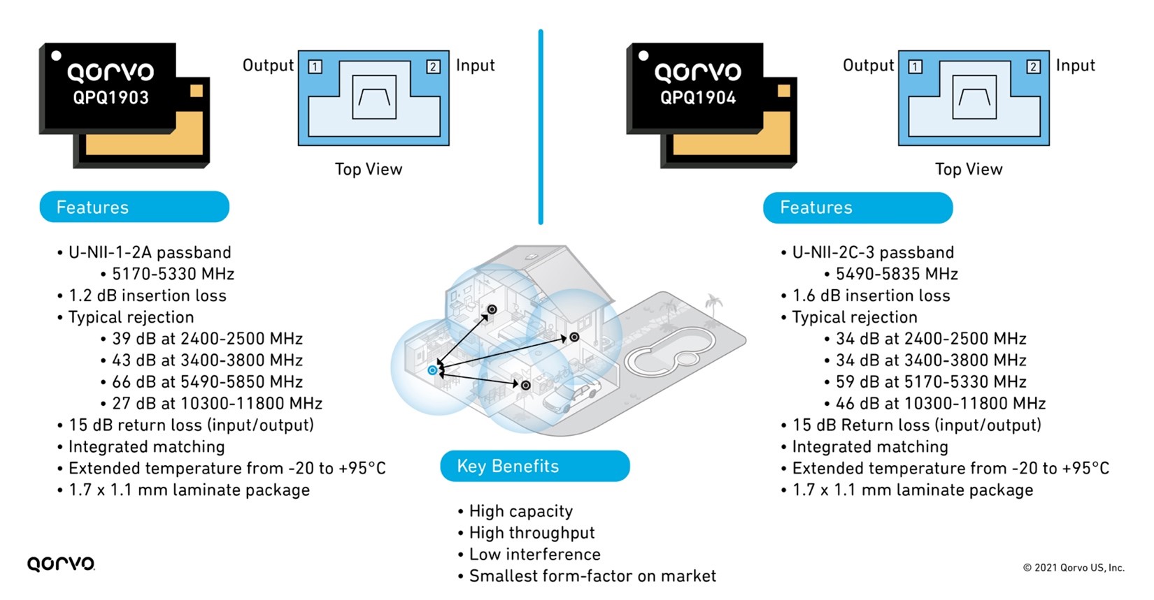
Figure 6: Features and benefits of QPQ1903 and QPQ1904
Not only are these filters providing benefits to the LNA, but they are small and perform well enough to install inside a tiny integrated Wi-Fi module package housing the LNA, switch, PA, and filter. Doing this drastically changes the end-product system layout making design easier and helps speed time-to-market. No longer are engineers burdened with matching and plugging individual passive and active components onto their PC board, but now they have all that done in these complex integrated modules called integrated front-end modules (iFEMs), creating a plug-and-play solution easily installed on their design.
A perfect example of this is the QPF7219 2.4 GHz iFEM, as seen in Figure 7. Qorvo has not only provided solutions with discrete edgeBoost BAW filters to increase output and capacity across all Wi-Fi channels. But Qorvo has gone a step further by including this filter inside an iFEM, our QPF7219, to provide customers with a drop-in pin-compatible replacement providing the same capacity and range performance outcome. This provides customers with design flexibility, board space in their design and is the first one of its kind on the market.
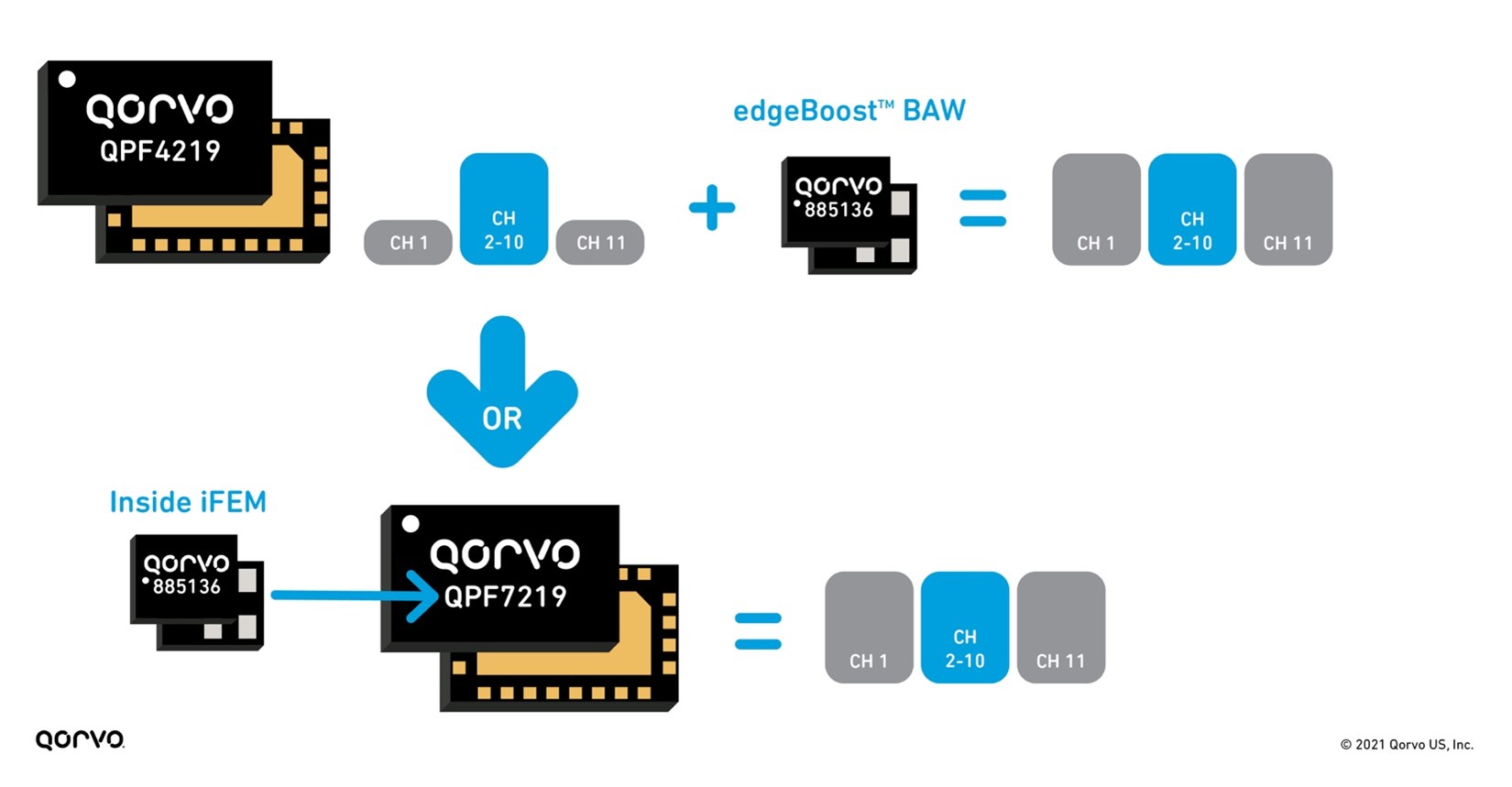
Figure 7: edgeBoost used as discrete and inside an iFEM
The need for smaller and sleeker product designs is always top of mind for Wi-Fi engineers. But to achieve the goal means component designers need to develop smaller products in many areas of the design, not just in one or two areas. From a tri-band Wi-Fi chip-set perspective, Qorvo has addressed this head-on. Qorvo has provided an entire group of iFEM alternatives to address the many signal transmit and receive lines in a product. This allows Wi-Fi design manufacturers to manage all the UNII and 2.4 GHz bands in a tri-band end-product design.
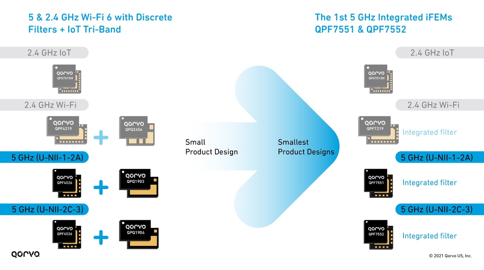
Figure 8: 2.4 & 5 GHz Wi-Fi 6 with IoT Tri-Band front-end solutions
This new design solution of combining the filter inside the iFEM equates to a smaller PC board and less shielding, as shown in Figure 9 below. Shielding matching and PC board space are expensive, not to mention the additional time associated with providing these materials. By placing all the RFFE materials inside a module, system designers can save cost, design faster, and get their products to market more quickly.
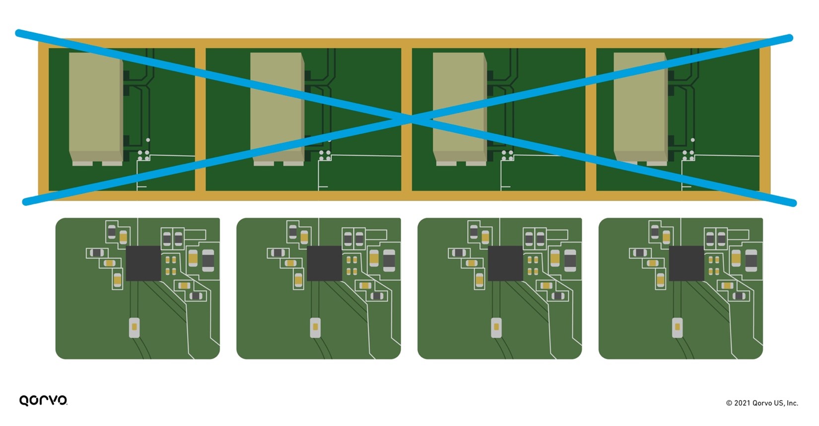
Figure 9: Putting the filter technology inside the iFEM removes shielding and reduces overall RFFE form-factor
As Wi-Fi system designers continue to be challenged with new specification requirements, they need newer or enhanced technologies to meet the need. By collaborating with our customers, we have provided state-of-the-art solutions to solve the tough thermal, performance, size, interference, capacity, throughput, and range difficulties seen by their end-customers. These solutions enable them to improve their designs to meet the Wi-Fi wave of today and in the future.
About the Author

Igor Lalicevic
Senior Marketing Manager, Wireless Connectivity Business Unit

Blog post from partner: https://www.gsitechnology.com/
Approximate Nearest-Neighbors for new voter party affiliation. Credit: http://scott.fortmann-roe.com/docs/BiasVariance.html
Introduction
The field of data science is rapidly changing as new and exciting software and hardware breakthroughs are made every single day. Given the rapidly changing landscape, it is important to take the appropriate time to understand and investigate some of the underlying technology that has shaped and will shape, the data science world. As an undergraduate data scientist, I often wish more time was spent understanding the tools at our disposal, and when they should appropriately be used. One prime example is the variety of options to choose from when picking an implementation of a Nearest-Neighbor algorithm; a type of algorithm prevalent in pattern recognition. Whilst there are a range of different types of Nearest-Neighbor algorithms I specifically want to focus on Approximate Nearest Neighbor (ANN) and the overwhelming variety of implementations available in python.
My first project with my internship at GSI Technology explored the idea of benchmarking ANN algorithms to help understand how the choice of implementation can change depending on the type and size of the dataset. This task proved challenging yet rewarding, as to thoroughly benchmark a range of ANN algorithms we would have to use a variety of datasets and a lot of computation. This would all prove to provide some valuable results (as you will see further down) in addition to a few insights and clues as to which implementations and implementation strategies might become industry standard in the future.
What Is ANN?
Before we continue its important to lay out the foundations of what ANN is and why is it used. New students to the data science field might already be familiar with ANN’s brother, kNN (k-Nearest Neighbors) as it is a standard entry point in many early machine learning classes.
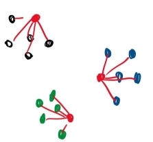
Red points are grouped with the five (K) closest points.
kNN works by classifying unclassified points based on “k” number of nearby points where distance is evaluated based on a range of different formulas such as Euclidean distance, Manhattan distance (Taxicab distance), Angular distance, and many more. ANN essentially functions as a faster classifier with a slight trade-off in accuracy, utilizing techniques such as locality sensitive hashing to better balance speed and precision. This trade-off becomes especially important with datasets in higher dimensions where algorithms like kNN can slow to a grueling pace.
Within the field of ANN algorithms, there are five different types of implementations with various advantages and disadvantages. For people unfamiliar with the field here is a quick crash course on each type of implementation:

- Brute Force; whilst not technically an ANN algorithm it provides the most intuitive solution and a baseline to evaluate all other models. It calculates the distance between all points in the datasets before sorting to find the nearest neighbor for each point. Incredibly inefficient.
- Hashing Based, sometimes referred to as LSH (locality sensitive hashing), involves a preprocessing stage where the data is filtered into a range of hash-tables in preparation for the querying process. Upon querying the algorithm iterates back over the hash-tables retrieving all points similarly hashed and then evaluates proximity to return a list of nearest neighbors.
- Graph-Based, which also includes tree-based implementations, starts from a group of “seeds” (randomly picked points from the dataset) and generates a series of graphs before traversing the graphs using best-first search. Through using a visited vertex parameter from each neighbor the implementation is able to narrow down the “true” nearest neighbor.
- Partition Based, similar to hashing, the implementation partitions the dataset into more and more identifiable subsets until eventually landing on the nearest neighbor.
- Hybrid, as the name suggests, is some form of a combination of the above implementations.
Because of the limitations of kNN such as dataset size and dimensionality, algorithms such as ANN become vital to solving classification problems with these kinds of constraints. Examples of these problems include feature extraction in computer vision, machine learning, and many more. Because of the prominence of ANN, and the range of applications for the technique, it is important to gauge how different implementations of ANN compare under different conditions. This process is called “Benchmarking”. Much like a traditional experiment we keep all variables constant besides the ANN algorithms, then compare outcomes to evaluate the performance of each implementation. Furthermore, we can take this experiment and repeat it for a variety of datasets to help understand how these algorithms perform depending on the type and size of the input datasets. The results can often be valuable in helping developers and researchers decide which implementations are ideal for their conditions, it also clues the creators of the algorithms into possible directions for improvement.
Open Source to the Rescue

Utilizing the power of online collaboration we are able to pool many great ideas into effective solutions
Beginning the benchmarking task can seem daunting at first given the scope and variability of the task. Luckily for us, we are able to utilize work already done in the field of benchmarking ANN algorithms. Aumüller, Bernhardsson, and Faithfull’s paper ANN-Benchmarks: A Benchmarking Tool for Approximate Nearest Neighbor Algorithms and corresponding GitHub repository provides an excellent starting point for the project.
Bernhardsson, who built the code with help from Aumüller and Faithfull, designed a python framework that downloads a selection of datasets with varying dimensionality (25 to nearly 28,000 dimensions) and size (few hundred megabytes to a few gigabytes). Then, using some of the most common ANN algorithms from libraries such as scikit-learn or the Non-Metric Space Library, they evaluated the relationship between queries-per-second and accuracy. Specifically, the accuracy was a measure of “recall”, which measures the ratio of the number of result points that are true nearest neighbors to the number of true nearest neighbors, or formulaically:
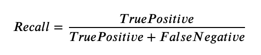
Intuitively recall is simply the correct predictions made by the algorithm, over the total number of correct predictions it could have made. So a recall of “1” means that the algorithm was correct in its predictions 100% of the time.
Using the project, which is available for replication and modification, I went about setting up the benchmark experiment. Given the range of different ANN implementations to test (24 to be exact), there are many packages that will need to be installed as well as a substantial amount of time required to build the docker environments. Assuming everything installs and builds as intended the environment should be ready for testing.
Results

After three days of run time for the GloVe-25-angular dataset, we finally achieved presentable results. Three days of runtime was quite substantial for this primary dataset, however as we soon learned this process can be sped up considerably. The implementation of the benchmark experiment defaults to running benchmarks twice and averaging the results to better account for system interruptions or other anomalies that might impact the results. If this isn’t an issue, computation time could be halved by only performing the benchmark tests once each. In our case we wanted to match Bernhardsson’s results so we computed the benchmark with the default setting of two runs per algorithm which produced the following:
Our results (top) and Bernhardsson’s results (bottom):

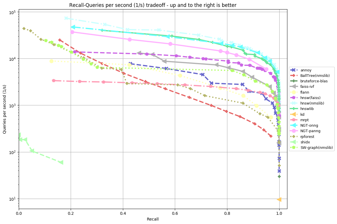
My Results vs Bernhardsson’s Results
As you can see from the two side by side plots of algorithm accuracy vs algorithm query speed there are some differences between my results and Bernhardsson’s. In our case, there are 18 functions plotted as opposed to 15 in the other. This is likely because the project has since been updated to include more functions following Bernhardsson’s initial tests. Furthermore, the benchmarking was performed on a different machine to Bernhardsson’s which likely produced some additional variability.
What we do see which is quite impressive is that many of the same algorithms that performed well for Bernhardsson also performed well in our tests. This suggests that across multiple benchmarks there are some clearly well-performing ANN implementations. NTG-onng, hnsw(nmslib) and hnswlib all performed exceedingly well in both cases. Hnsw(nmslib) and hnswlib both belong to the Hierarchical Navigable Small World family, an example of a graph-based implementation for ANN. In fact, many of the algorithms tested, graph-based implementations seemed to perform the best. NTG-onng is also an example of a graph-based implementation for ANN search. This suggests that graph-based implementations of ANN algorithms for this type of dataset perform better than other competitors.
In contrast to the well-performing graph-based implementations, we can see BallTree(nmslib) and rpforest both of which in comparison are quite underwhelming. BallTree and rpforest are examples of tree-based ANN algorithms (a more rudimentary form of a graph-based algorithm). BallTree specifically is a hybrid tree-partition algorithm combining the two methods for the ANN process. It is likely a series of reasons that cause these two ANN algorithms to perform poorly when compared to HNSW or NTG-onng. However, the main reason seems to be that tree-based implementations execute slower under the conditions of this dataset.
Although graph-based implementations outperform other competitors it is worth noting that graph-based implementations suffer from a long preprocessing phase. This phase is required to construct the data structures necessary for the computation of the dataset. Hence using graph-based implementations might not be ideal under conditions where the preprocessing stage would have to be repeated.
One advantage our benchmark experiment had over Bernhardsson’s is our tests were run on a more powerful machine. Our machine (see appendix for full specifications) utilized the power of 2 Intel Xeon Gold 5115’s, an extra 32 GBs of DDR4 RAM totaling 64 GBs, and 960 GBs of solid-state disk storage which differs from Bernhardsson’s. This difference likely cut down on computation time considerably, allowing for faster benchmarking.
A higher resolution copy of my results can be found in the appendix.
Conclusion and Future Work

Further benchmarking for larger deep learning datasets would be a great next step.
Overall, my first experience with benchmarking ANN algorithms has been an insightful and appreciated learning opportunity. As we discussed above there are some clear advantages to using NTG-onng and hnsw(nmslib) on low dimensional smaller datasets such as the glove-25-angular dataset included with Erik Bernhardsson’s project. These findings, whilst coming at an immense computational cost, are none the less useful for data scientists aiming to tailor their use of ANN algorithms to the dataset they are utilizing.
Whilst the glove-25-angular dataset was a great place to start I would like to explore how these algorithms perform on even larger datasets such as the notorious deep1b (deep one billion) dataset which includes one billion 96 dimension points in its base set. Deep1b is an incredibly large file that would highlight some of the limitations as well as the advantages of various ANN implementations and how they trade-off between query speed and accuracy. Thanks to the hardware provided by GSI Technology this experiment will be the topic of our next blog.
Appendix
- Computer specifications: 1U GPU Server 1 2 Intel CD8067303535601 Xeon® Gold 5115 2 3 Kingston KSM26RD8/16HAI 16GB 2666MHz DDR4 ECC Reg CL19 DIMM 2Rx8 Hynix A IDT 4 4 Intel SSDSC2KG960G801 S4610 960GB 2.5″ SSD.
- Full resolution view of my results:
Sources
- Aumüller, Martin, Erik Bernhardsson, and Alexander Faithfull. “ANN-benchmarks: A benchmarking tool for approximate nearest neighbor algorithms.” International Conference on Similarity Search and Applications. Springer, Cham, 2017.
- Liu, Ting, et al. “An investigation of practical approximate nearest neighbor algorithms.” Advances in neural information processing systems. 2005.
- Malkov, Yury, et al. “Approximate nearest neighbor algorithm based on navigable small-world graphs.” Information Systems 45 (2014): 61–68.
- Laarhoven, Thijs. “Graph-based time-space trade-offs for approximate near neighbors.” arXiv preprint arXiv:1712.03158 (2017).