A Beginner’s Guide to Segmentation in Satellite Images: Walking through machine learning techniques for image segmentation and applying them to satellite imagery
Blog from: https://www.gsitechnology.com/
In my first blog, I walked through the process of acquiring and doing basic change analysis on satellite data. In this post, I’ll be discussing image segmentation techniques for satellite data and using a pre-trained neural network from the SpaceNet 6 challenge to test an implementation out myself.
What is image segmentation?
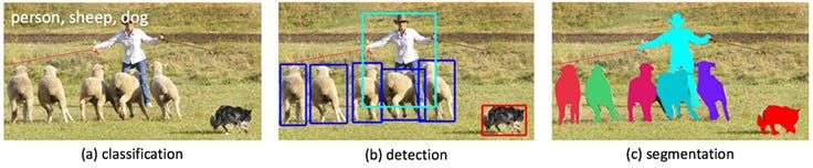
As opposed to image classification, in which an entire image is classified according to a label, image segmentation involves detecting and classifying individual objects within the image. Additionally, segmentation differs from object detection in that it works at the pixel level to determine the contours of objects within an image.
In the case of satellite imagery, these objects may be buildings, roads, cars, or trees, for example. Applications of this type of aerial imagery labeling are widespread, from analyzing traffic to monitoring environmental changes taking place due to global warming.
The SpaceNet project’s SpaceNet 6 challenge, which ran from March through May 2020, was centered on using machine learning techniques to extract building footprints from satellite images—a fairly straightforward problem statement for an image segmentation task. Given this, the challenge provides us with a good starting point from which we can begin to build understanding of what is an inherently advanced process.
I’ll be exploring approaches taken to the SpaceNet 6 challenge later in the post, but first, let’s explore a few of the fundamental building blocks of machine learning techniques for image segmentation to uncover how code can be used to detect objects in this way.
Convolutional Neural Networks (CNNs)
You’re likely familiar with CNNs and their association with computer vision tasks, particularly with image classification. Let’s take a look at how CNNs work for classification before getting into the more complex task of segmentation.
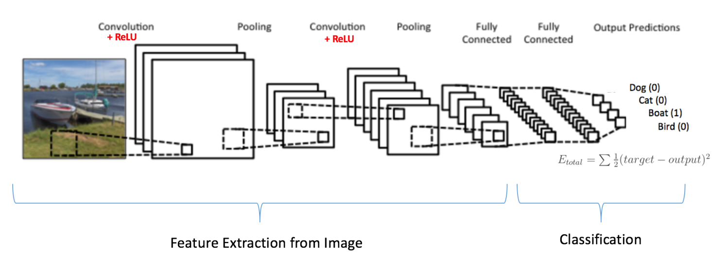
As you may know, CNNs work by sliding (i.e. convolving) rectangular “filters” over an image. Each filter has different weights and thus gets trained to recognize a particular feature of an image. The more filters a network has—or the deeper a network is—the more features it can extract from an image and thus the more complex patterns it can learn for the purpose of informing its final classification decision. However, given that each filter is represented by a set of weights to be learned, having lots of filters of the same size as the original input image makes training a model quite computationally expensive. It’s largely for this reason that filters typically decrease in size over the course of a network, while also increasing in number such that fine-grained features can be learned. Below is an example of what the architecture for an image classification task might look like:
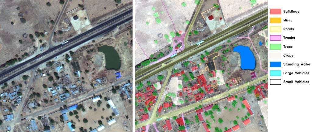
As we can see, the output of the network is a single prediction for a class label, but what would the output be for a segmentation task, in which an image may contain objects of multiple classes in different locations? Well, in such a case, we want our network to produce a pixel-wise map of classifications like the following:
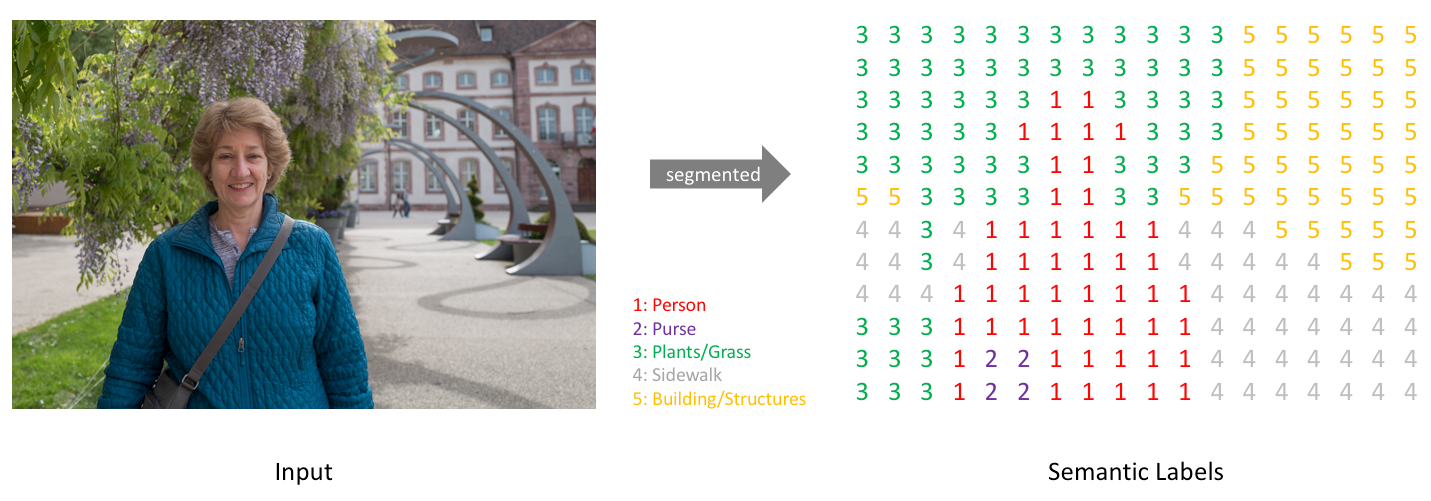
An image and its corresponding simplified segmentation map of pixel class labels. Source
To generate this, our network has a one-hot-encoded output channel for each of the possible class labels:

These maps are then collapsed into one by taking the argmax at each pixel position.
The tricky part of achieving this segmentation is that the output has to be aligned with the input image—we can’t follow the exact same downsampling architecture that we use in a classification task to promote computational efficiency because the size and locality of the class areas must be preserved. The network also needs to be sufficiently deep to learn detailed enough representations of each of the classes such that it can distinguish between them. One of the most popular kinds of architecture for meeting these demands is what is known as a Fully Convolutional Network.
Fully Convolutional Networks (FCNs)
FCN’s get their name from the fact that they contain no fully-connected layers, that is, they are fully convolutional. This structure was first proposed by Long et al. in a 2014 paper, which I aim to summarize key points of here.
With standard CNNs, such as those used in image classification, the first layer of the network is fully-connected, meaning it has the same dimensions as the input image; this means that the size of the first layer must be fixed to align with the input image. Not only does this render the network inflexible to inputs of different sizes, it also means that the network uses global information (i.e. information from the entire image) to make its classification decision, which does not make sense in the context of image segmentation in which our goal is to assign different class labels to different regions of the image. Convolutional layers, on the other hand, are smaller than the input image so that they can slide over it—they operate on local input regions.
In short, FCNs replace the fully-connected layers of standard CNNs with convolutional layers with large receptive fields. The following figure illustrates this process. We see how a standard CNN for classification of a cat-only image can be transformed to output a heatmap for localizing the cat in the context of a larger image:
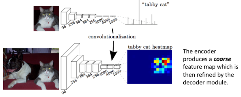
Moving through the network, we can see that the size of the layers getting smaller and smaller for the sake of learning finer features in a computationally efficient manner—a process known as “downsampling.” Additionally, we notice that the cat heatmap is of coarser resolution than the input image. Given these factors, how does the coarse feature map get translated back to the size of the input image at a high enough resolution such that the pixel classifications are meaningful? Long et al. used what is known as learned upsampling to expand the feature map back to the same size as the input image and a process they refer to as “skip layer fusion” to increase its resolution. Let’s take a closer look at these techniques.
Demystifying Learnable Upsampling
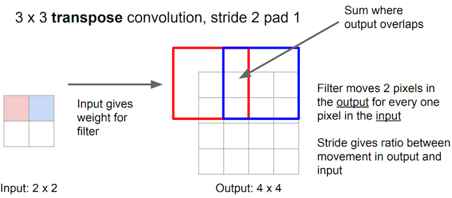
Prior approaches to upsampling relied on hard-coded interpolation methods, but Long et al. proposed a technique that uses transpose convolution to upsample small feature maps in a learnable way. Recall the way that normal convolution works:
The filter represented by the shaded area slides over the blue input feature map, computing dot products at each position to be recorded in the green output feature map. The weights of the filter are what is being learned by the network during training.
Transpose convolution works differently: the filter’s weights are all multiplied by the scalar value of the input pixel it is positioned over, and these values get projected to the output feature map. Where filter projections in the output map overlap, their values are added.
Long et al. use this technique to upsample the feature map rendered by network’s downsampling layers in order to translate its coarse output back to pixels that align with those of the input image, such that the network’s architecture looks like this:
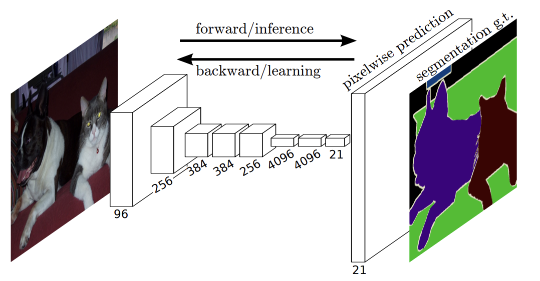
An example of a final upsampling layer appended to the downsampling path to render a full-sized segmentation map. Note that the final feature map has 21 channels, representing the number of classes for the particular segmentation challenge being explored in the paper. Source
However, simply adding one of these transpose convolutional layers at the end of the downsampling layers yields spatially imprecise results, as the large stride required to make the output size match the input’s (32 pixels, in this case) limits the scale of detail the upsampling can achieve:
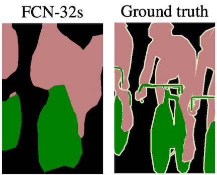
The upsampled segmentation map (left) is appropriately scaled to the input image but lacks spatial precision. Source
Luckily, this lack of spatial precision can be somewhat mitigated by “fusing” information from layers with different strides, as we’ll now discuss.
Skip Layer Fusion
As previously mentioned, a network must be deep enough to learn detailed features such that it can make faithful classification predictions; however, zeroing in closely on any one part of an image comes at the cost of losing spatial context of the image as a whole, making it harder to localize your classification decision in the process of zooming back out. This is the inherent tension at play in image segmentation tasks, and one that Long et al. work to resolve using skip connections.
In neural networks, a skip connection is a fusion between non-adjacent layers; in this case, skip connections are used to transfer local information by summing feature maps from the downsampling path with feature maps from the upsampling path. Intuitively, this makes sense: with each step we take through the downsampling path of the network, global information gets lost as we zoom into a particular area of the image and the feature maps get coarser, but once we have gone sufficiently deep to make an accurate prediction, we wish to zoom back and localize it, which we can do utilizing information stored in the higher resolution feature maps from the downsampling path of the network. Let’s take a more in depth look at this process by referencing the architecture Long et al. use in their paper:
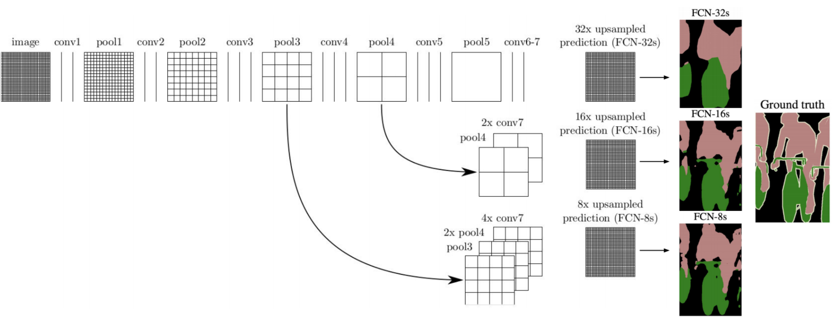
Visualization of skip connections (left arrows) in a network and their effect on the granularity of resulting segmentation maps. Source (modified)
Across the top of the image is the network’s downsampling path, which we can see follows a pattern of two or three convolutions followed by a pooling layer. conv7 represents the coarse feature map generated at the end of the downsampling path, akin to the cat heatmap we saw earlier. The “32x upsampled prediction” is the result of the first architecture without any skip connections, accomplishing all of the necessary upsampling with a single transpose convolutional layer of a 32 pixel stride.
Let’s walk through the “FCN-16s” architecture, which involves one skip connection (see the second row of the diagram). Though it is not visualized, a 1×1 convolution layer is added on top of the “pool4” feature map to produce class predictions for all its pixels. But the network does not end there—it proceeds to downsample by a factor of 2 once more to produce the “conv7” class prediction map. Since the conv7 map is of half the dimensionality of the pool4 map, it is upsampled by a factor of 2 and its predictions are added to those of the pool4, producing a combined prediction map. This result is upsampled via a transpose convolution with a stride of 16 to yield the final “FCN-16s” segmentation map, which we can see achieves better spatial resolution than the FCN-32s map. Thus, although the conv7 predictions experience the same amount of upsampling in the end as in the FCN-32s architecture (given that 2x upsampling followed by 16x upsampling = 32x upsampling), factoring the predictions from the pool4 layer improves the result greatly. This is because pool4 reintroduces valuable spatial information from the input image into the equation—information that otherwise gets lost in the additional downsampling operation for producing conv7. Looking at the diagram, we can see that the “FCN-8s” architecture follows a similar process, but this time a skip connection is also added from the “pool3” layer, which we see yields an even higher fidelity segmentation map.
FCNs—Where to go from here?
FCNs were a big step in semantic segmentation for their ability to factor in both deep, semantic information and fine, appearance information to make accurate predictions via an “encoding and decoding” approach. But the original architecture proposed by Long et al. still falls short of ideal. For one, it results in somewhat poor resolution at segmentation boundaries due to loss of information in the downsampling process. Additionally, overlapping outputs of the transpose convolution operation discussed earlier can cause undesirable checkerboard-like patterns in the segmentation map, which we see an example of below:
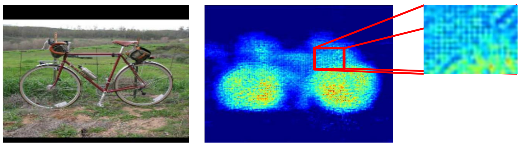
Criss-crossing patterns in a segmentation heatmap resulting from overlapping transpose convolution outputs. Source
Many models have built upon the promising baseline FCN architecture, seeking to iron out its shortcomings, “U-net” being a particularly notable iteration.
U-Net—An Optimized FCN
U-net was first proposed in a 2015 paper as an FCN model for use in biomedical image segmentation. As the paper’s abstract states, “The architecture consists of a contracting path to capture context and a symmetric expanding path that enables precise localization,” yielding a u-shaped architecture that looks like this:
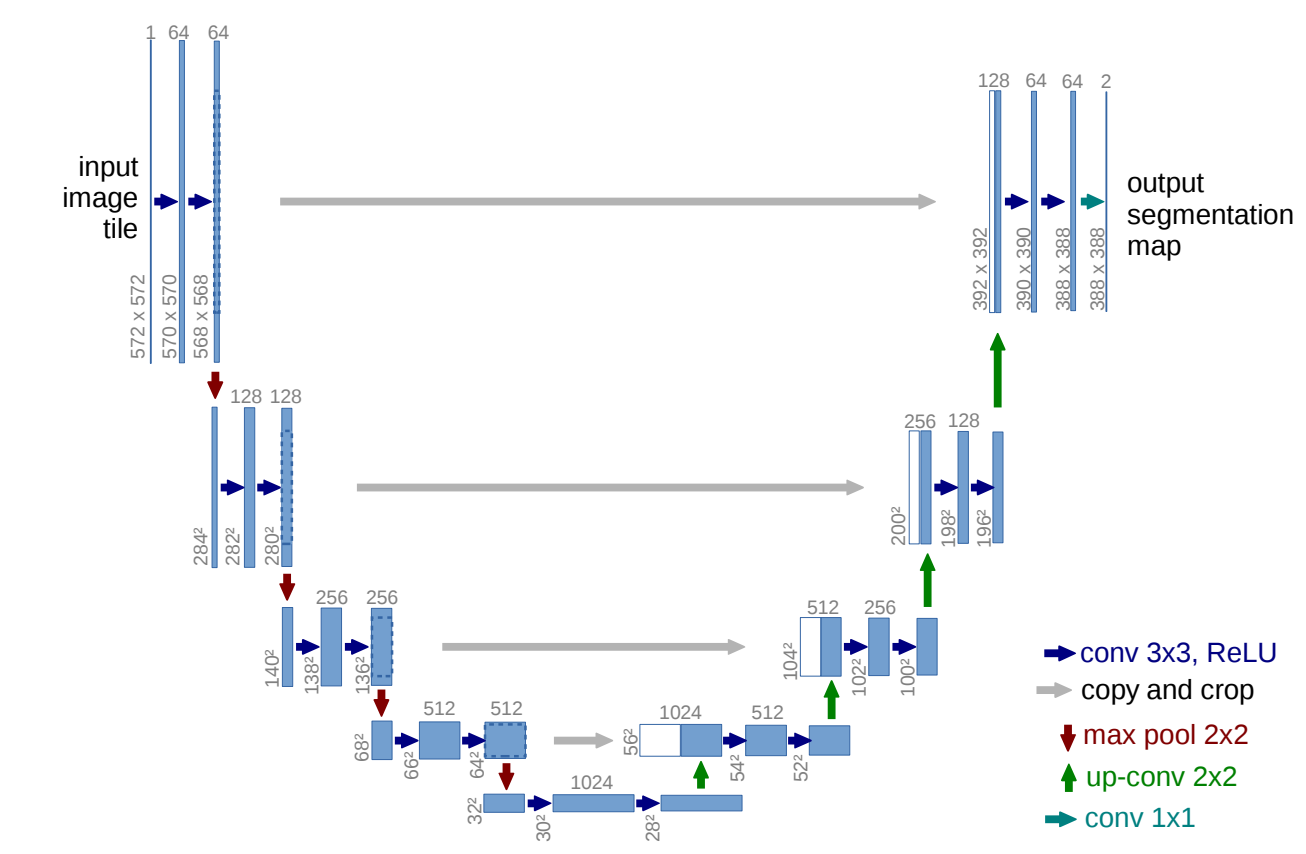
An implementation of the U-net architecture. Numbers at the top of the feature maps denote their number of channels, numbers at the bottom left denote their x-y-size. The white feature maps represent are copies from the downsampling path, which we can see get concatenated to feature maps in the upsampling path. Source
We can see that the network involves 4 skip connections—after each transpose convolution (or “up-conv”) in the upsampling path, the resulting feature map gets concatenated with one from the downsampling path. Additionally, we see that the feature maps in the upsampling path have a larger number of channels than in the baseline FCN architecture for the purpose of passing more context information to higher resolution layers.
U-net also achieves better resolution at segmentation boundaries by pre-computing a pixel-wise weight map for each training instance. The function used to compute the map places higher weights on pixels along segmentation boundaries. These weights are then factored into the training loss function such that boundary pixels are given higher priority for being classified correctly.
We can see that the original U-net architecture yields quite fine-grained results in its cellular segmentation tasks:
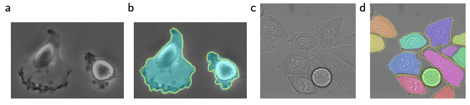
U-net segmentations results in images b and d, with ground truth boundaries outlined in yellow. Source
The development of U-net yet was another milestone in the field of computer vision, and five years later, models continue to expound upon its u-shaped architecture to achieve better and better results. U-net lends itself well to satellite imagery segmentation, which we will circle back to soon in the context of the SpaceNet 6 challenge.
Further Developments in Image Segmentation
We’ve now walked through an evolution of a few basic image segmentation concepts—of course, only scratching the surface of a topic at the center of a vast, rapidly evolving field of research. Here is a list of a few other interesting image segmentation concepts and applications, with links should you wish to explore them further:
- Instance segmentation is a hybrid of object detection and image segmentation in which pixels are not only classified according to the class they belong to, but individual objects within these classes are also extracted, which is useful when it comes to counting objects, for example.
- Techniques for image segmentation extend to video segmentation as well; for example, Google AI uses an “hourglass segmentation network architecture” inspired by U-net for real-time foreground-background separation in YouTube stories.
- Clothing image segmentation has been used to help retailers match catalogue items with physical items in warehouses for more efficient inventory management.
- Segmentation can be applied to 3D volumetric imagery as well, which is particular useful in medical applications; for example, research has been done on using it to monitor the development of brain lesions in stroke patients.
- Many tools and packages have been developed to make image segmentation accessible to people of various skill levels. For instance, here is an example that uses Python’s PixelLib library to achieve 150-class segmentation with just 5 lines of code.
Now, let’s walk through actually implementing a segmentation network ourselves using satellite images and a pre-trained model from the SpaceNet 6 challenge.
The SpaceNet 6 Challenge
The task outlined by the SpaceNet challenge is to use computer vision to automatically extract building footprints from satellite images in the form of vector polygons (as opposed to pixel maps). In the challenge, predictions generated by a model are determined viable or not by calculating their intersection over union with ground truth footprints. The model’s f1 score over all the test images is calculated according to these determinations, serving as the metric for the competition.
The training dataset consists of a mix of mostly synthetic aperture radar (SAR) and a few electro-optical (EO) 0.5m resolution satellite images collected by Capella Space over Rotterdam, the Netherlands. The testing dataset contains only SAR images (for further explanation on SAR imagery, take a look at my last blog). The dataset being structured in this way makes the challenge particularly relevant to real-world applications, as SpaceNet explains, it is meant to “mimic real-world scenarios where historical optical data may be available, but concurrent optical collection with SAR is often not possible due to inconsistent orbits of the sensors, or cloud cover that will render the optical data unusable.”
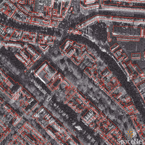
An example of a SAR image from the SpaceNet 6 dataset, with building footprint annotations shown in red. Source
More information on the dataset, including instructions for downloading it, can be found here. Additionally, SpaceNet released a baseline model, for which they provide explanation and code. Let’s explore the architecture of this model before implementing it to make predictions ourselves.
The Baseline Model
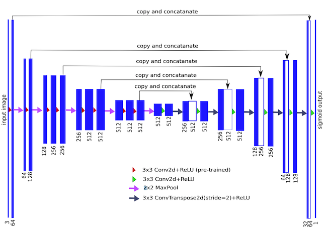
TernausNet architecture. Source
The architecture SpaceNet uses as its baseline is called TernausNet, a variant of U-Net with a VGG11 encoder. VGG is a family of CNNs, VGG11 being one with 11 layers. TernausNet uses a slightly modified version of VGG11 as its encoder (i.e. downsampling path). The network’s upsampling path mirrors its downsampling path, with 5 skip connections linking the two. TernausNet improves upon U-Net’s performance by initializing the network with weights that were pre-trained on Kaggle’s Carvana dataset. Using a model pre-trained on other data can reduce training time and overfitting—an approach known as transfer learning. In fact, SpaceNet’s baseline takes advantage of transfer learning again by first training on only the optical portion of the training dataset, then using the weights it finds through this process as the initial weights in its final training pass on the SAR data.
Even with these applications of transfer learning, though, training the model on roughly 24,000 images is still a very time intensive process. Luckily, SpaceNet provides the weights for the model at its highest scoring epoch, which allow us to get the model up and running fairly easily.
Making Predictions from the Baseline Model
Step-by-step instructions for deploying the baseline model can be found in this blog. In short, the process involves spinning up an AWS Elastic Cloud Compute (EC2) instance to gain access to GPUs for more timely computation and loading the challenge’s Amazon Machine Image (AMI), which is pre-loaded with the software, baseline model and dataset. Keep in mind that the dataset is very large, so downloads may take some time.
Once your downloads are complete, you can find the PyTorch code defining the baseline model in model.py. baseline.py takes care of image preprocessing and running training and testing operations. The weights of the pre-trained model with the best scoring epoch are found in the weights folder and are loaded when test.sh is run.
When we run an image through the model, it outputs a series of coordinates that define the boundaries of the building footprints we are looking to find as well as a mask on which these footprints are plotted. Let’s walk through the process of visualizing an image and its mask side-by-side to get a sense of how effective the baseline model is at extracting building footprints. Code for producing the following visualizations can be found here.
Getting a coherent visual representation of the SAR data is somewhat trickier than expected. This is because each pixel in a given image is assigned 4 values, corresponding to 4 polarizations of data in the X-band of the electromagnetic spectrum—HH, HV, VH and VV. In short, signals transmitted and received from a SAR sensor come in both horizontal and vertical polarization states, so each channel corresponds to a different combination of the transmitted and received signal types. These 4 channels don’t translate to the 3 RGB channels we expect for rendering a typical image. Here’s what it looks like when we select the channels one-by-one and visualize them in grayscale:
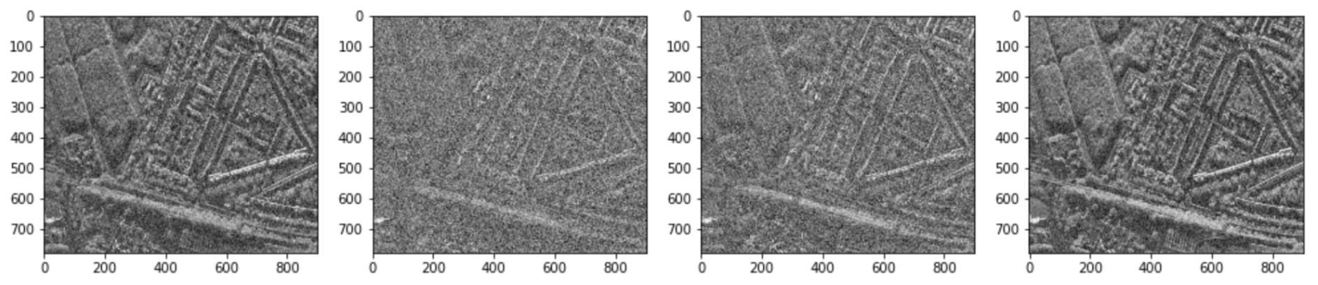
Visual representations of the 4 polarizations of a single SAR image. Image by author
Notice that each of the 4 polarizations captures a slightly different representation of the same area of land. We can combine these representations to produce a single-channel span image to plot alongside the building footprint mask the model generated, which we convert to binary to make the boundaries more clear. With this, we can see that the baseline model did recognize the general shapes of several buildings:
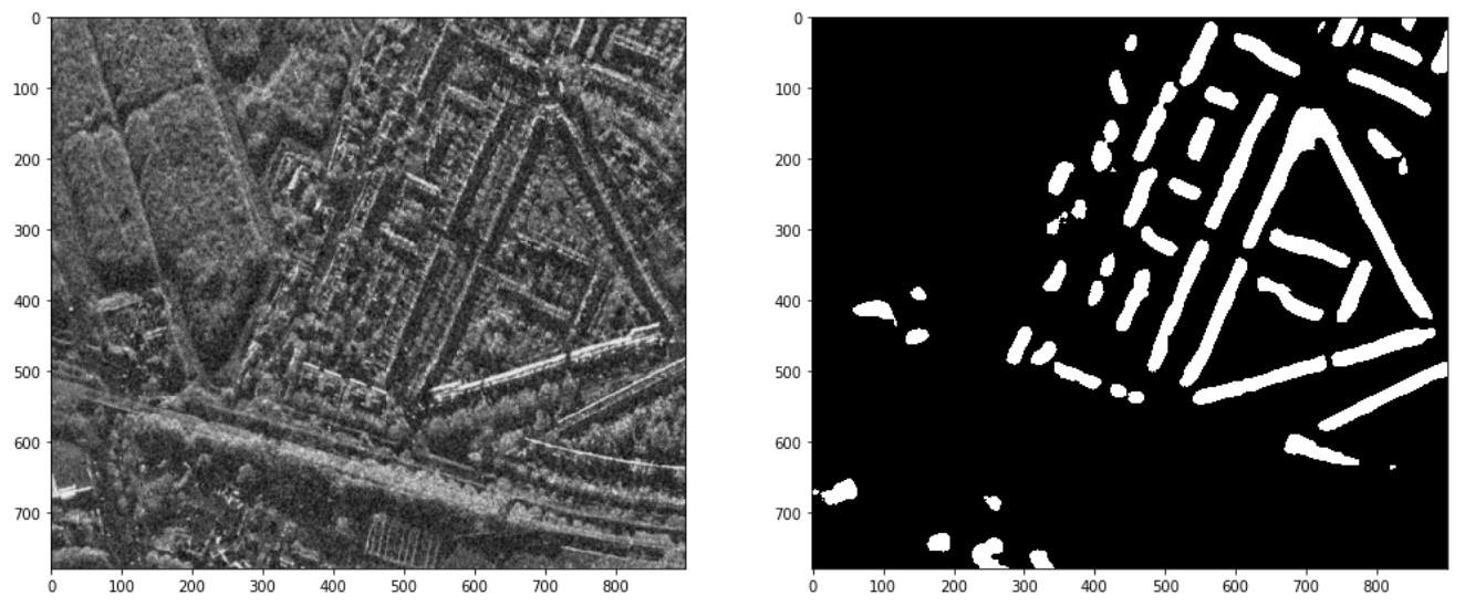
A visualization of the combined spectral bands of a SAR test image and the corresponding building footprint mask generated by the baseline model. Image by author
It is pretty cool to see the basic structures we’ve discussed in this post in action here, producing viable image segmentation results. But, it’s also clear that there is room for improvement upon this baseline architecture—indeed, it only achieves an f1 score of 0.21 on the test set.
Conclusion
The SpaceNet 6 challenge wrapped up in May, with the winning submission achieving an f1 score of 0.42—double that of the baseline model. More details on the outcomes of the challenge can be found here. Notably, all of the top 5 submissions implemented some variant of U-Net, an architecture that we now have a decent understanding of. SpaceNet will be releasing these highest performing models on GitHub in the near future and I look forward to trying them out on time series data to do some exploration with change detection in a future post.
Lastly, I’m very thankful for the thorough and timely assistance I received from Capella Space for writing this—their insight into the intricacies of SAR data as well as recommendations and code for processing it were integral to this post.
References
- https://missinglink.ai/guides/computer-vision/image-segmentation-deep-learning-methods-applications/
- https://ujjwalkarn.me/2016/08/11/intuitive-explanation-convnets/
- https://engineering.matterport.com/splash-of-color-instance-segmentation-with-mask-r-cnn-and-tensorflow-7c761e238b46
- https://arxiv.org/abs/1411.4038
- https://www.youtube.com/watch?v=nDPWywWRIRo&list=PLC1qU-LWwrF64f4QKQT-Vg5Wr4qEE1Zxk&index=11
- http://deeplearning.net/tutorial/fcn_2D_segm.html
- https://www.topbots.com/semantic-segmentation-guide/
- https://arxiv.org/pdf/1505.04597.pdf
- https://medium.com/the-downlinq/spacenet-6-announcing-the-winners-df817712b515
- https://simularity.com/using-aisaroptical-to-find-the-invisible/