Blog post from Knowles Precision Devices. Starvoy represents Knowles Precision Devices across Canada, for further information on their range of highly engineered Capacitors and Microwave to Millimeter Wave components for use in critical applications in military, medical, electric vehicle, and 5G market segments.

To protect people and critical equipment, military-grade electronic devices must be designed to function reliably while operating in incredibly harsh environments. Therefore, instead of continuing to use traditional silicon semiconductors, in recent years, electronic device designers have started to use wide band-gap (WBG) materials such as silicon carbide (SiC) to develop the semiconductors required for military device power supplies. In general, WBG materials can operate at much higher voltages, have better thermal characteristics, and can perform switching at much higher frequencies. Therefore, SiC-based semiconductors provide superior performance compared to silicon, including higher power efficiency, higher switching frequency, and higher temperature resistance as shown in Figure 1.

As the shift to using SiC-based semiconductors continues, other board-level components, such as capacitors, must change as well. For example, as systems operate at higher frequencies, the capacitance needed decreases, leading to many instances where film capacitors can be replaced by ceramic capacitors.

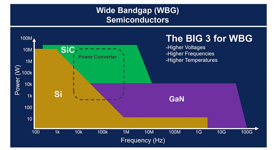
Figure 1. A comparison of traditional silicon semiconductor material to WBG materials such as SiC and GaN. Source.

Why You Need to Use Ceramic Capacitors with Your SiC Semiconductors

In general, ceramic capacitors are small and lightweight, making ceramic capacitors an ideal option for military applications where space and weight are at a premium. When using SiC semiconductors specifically, since the switching speeds are quite fast, high-frequency noise and voltage spikes will occur. Ceramic capacitors are needed to filter out this noise. And for high-frequency power supplies applications, ceramic capacitors are a preferred option because these components have a high self-resonant frequency, low equivalent series resistance (ESR), and high thermal stability.

Knowles Precision Devices: Your Military-Grade Ceramic Capacitor Experts

As a manufacturer of specialty ceramic capacitors, Knowles provide a variety of high-performance, high-reliability capacitors that are well-suited for military applications. At a basic level, they build all of their catalog and custom passive components to MIL-STD-883, a standard that “establishes uniform methods, controls, and procedures for testing microelectronic devices suitable for use within military and aerospace electronic systems.” We also hold the internationally recognized qualification for surface mount ceramic capacitors tested in accordance with the requirements of IECQ-CECC QC32100 as well as a variety of other quality certificates and approvals. For their high-reliability capacitors, they go above and beyond these quality standards and ensure components are burned-in at elevated voltage and temperature levels and are 100 percent electrically inspected to conform to strict performance criteria

Please contact the Starvoy team for further information, or to discuss your requirements.