Original post from: https://www.qorvo.com/design-hub/blog/what-designers-need-to-know-to-achieve-wi-fi-tri-band-gigabit-speeds-and-high-throughput
Engineers are always looking for the simplest solution to complex system design challenges. Look no further for answers in the U-NII 1-8, 5 and 6 GHz realm. Here we review how state-of-the-art bandBoost™ filters help increase system design capacity and throughput, offering engineers an easy, flexible solution to their complex designs, while at the same time helping to meet those tough final product compliance requirements.
A Summary of Where We are Today in Wi-Fi
Wi-Fi usage has grown exponentially over the years. Most recently, it has skyrocketed upward to unimaginable levels — driven by the pandemic of 2020 due to work from home, school requirements, gaming advancements, and, of course, 5G. According to Statista, the first weeks of March 2020 saw an 18 percent increase in in-home data usage compared to the same period in 2019, with average daily data usage rates exceeding 16.6 GB.
With this increase in usage comes an increase in expectations to access Wi-Fi anywhere — throughout the home, both inside and out, and at work. Meeting these expectations requires more wireless backhaul equipment to transport data between the internet and subnetworks. It also requires advancements in existing technology to reach the capacity, range, signal reliability and the rising number of new applications wireless service providers are seeing. Figure 1 shows the exponential increase in wireless applications — from email to videoconferencing, smart home capabilities, gaming and virtual reality — as wireless technology continues to advance.
Go In Depth:
- Read Qorvo’s white paper that provides a play-by-play of how Wi-Fi has evolved over the past 20 years.
- Learn more about our industry-leading BAW Filter solutions.
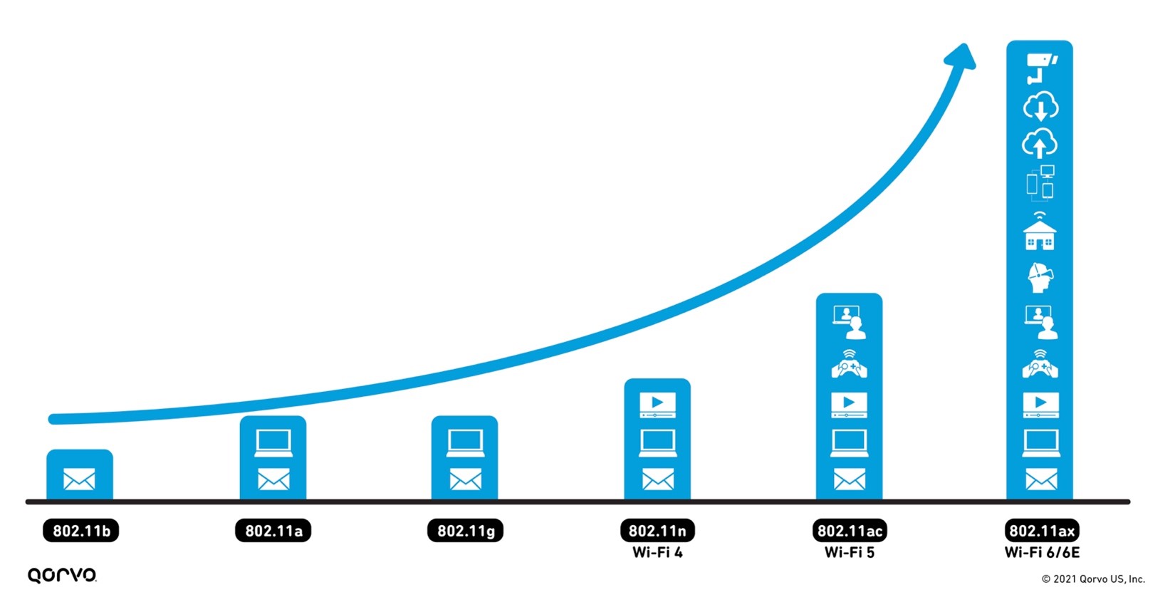
Figure 1: The advancement of Wi-Fi
The 802.11 standard has now advanced onto Wi-Fi 6 and Wi-Fi 6E, providing service beyond 5 GHz and into the 6 GHz area up to 7125 GHz, as shown in Figure 2. This higher frequency range increases our video capacities for our security systems and streaming.
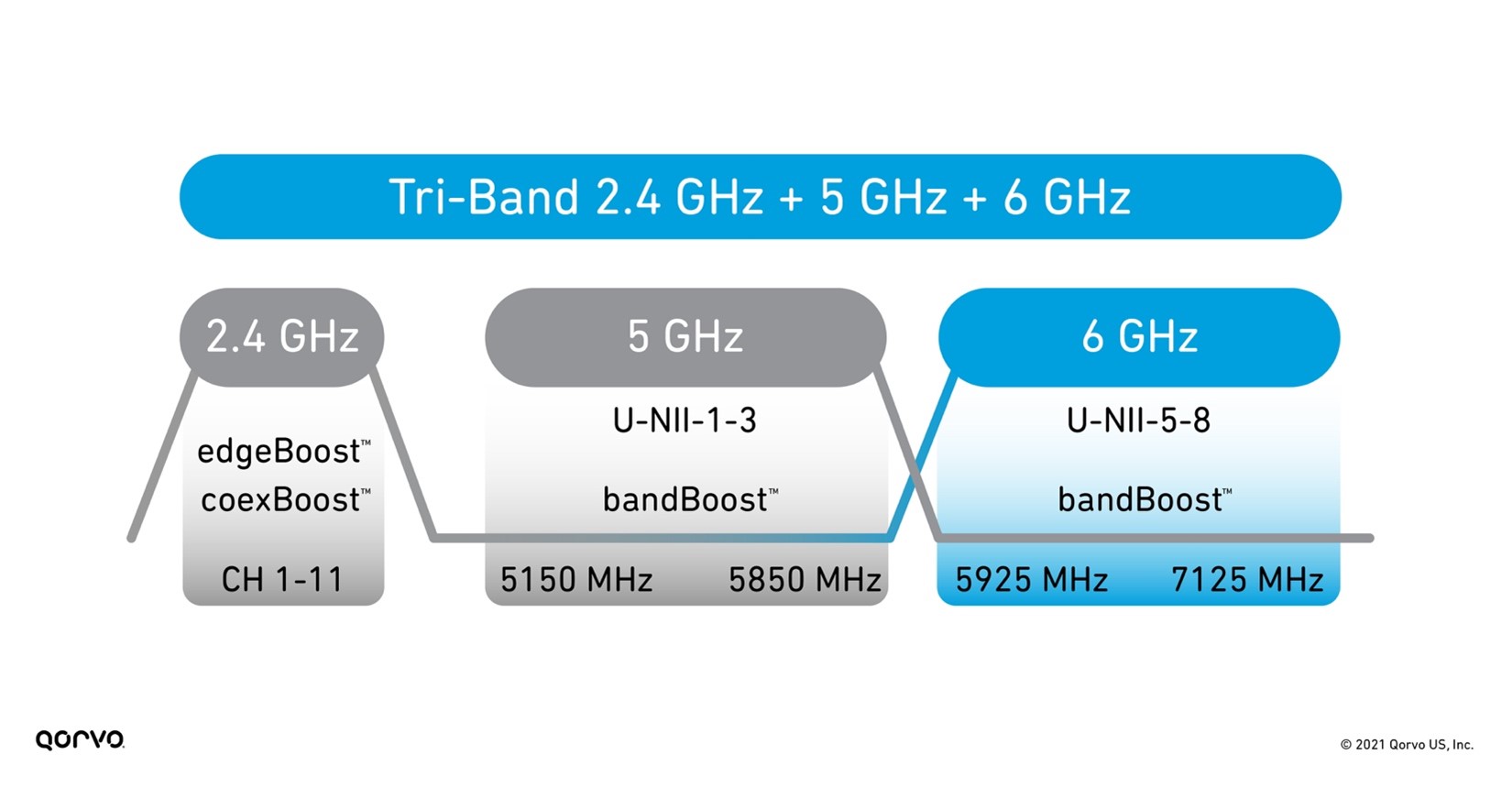
Figure 2: Tri-Band Wi-Fi frequency bands
However, working in higher frequency ranges can bring challenges such as more signal attenuation and thermal increases — especially when trying to meet the requirements of small form factors. To meet these challenges head-on, RF front-end (RFFE) engineers need to take existing technology to another level. One of those advancements has been in BAW filter technology now being used heavily in Wi-Fi system designs.
As shown in Figure 3 below, Qorvo has three BAW filter variants that boost overall Wi-Fi performance, maximize network capacity, increase RF range, and mitigate interference between the many different in-home radios operating simultaneously.
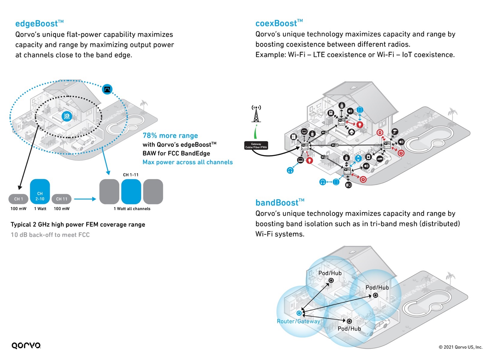
Figure 3: bandBoost, edgeBoost, and coexBoost filter technology performance
5 & 6 GHz bandBoost Filters
In a previous blog post called An Essential Part of The Wi-Fi Tri-Band System – 5.2 GHz RF Filters, we explored how using bandBoost filters like the Qorvo QPQ1903 and QPQ1904 can help reduce design complexity and help with coexistence. We also explored how these bandBoost filters provide high isolation, helping to reduce that function on the antenna design, allowing for less expensive antennas. Therefore, the RFFE isolation parameter no longer needs to rest entirely on the antenna. This reduces antenna and shielding costs – providing up to a 20 percent cost reduction.
These bandBoost BAW filters play a key role in separating the U-NII-2A band from the U-NII-2C band, which only has a bandgap of 120 MHz, as shown in Figure 4. Using these filters, we can attain Wi-Fi coverage reaching every corner of the home with the highest throughput and capacity. Using this solution in a Wi-Fi system design has shown increases in capacity for the end user up to 4-times.
Unlicensed National Information Infrastructure (U-NII)
The U-NII radio band, as defined by the United States Federal Communications Commission, is part of the radio frequency spectrum used by WLAN devices and by many wireless ISPs.
As of March 2021, U-NII consists of eight ranges. U-NII 1 through 4 are for 5 GHz WLAN (802.11a and newer), and 5 through 8 are for 6 GHz WLAN (802.11ax) use. U-NII 2 is further divided into three subsections: A, B and C.
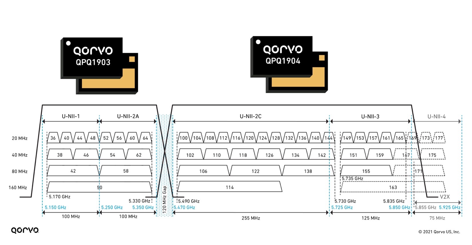
Figure 4: 5 GHz bandBoost filters and U-NII 1-4 bands
These filters are much smaller than legacy filters on the market used in Wi-Fi applications — allowing for more compact tri-band radios. They also have superior isolation achieving greater than 80 dBm system isolation for designers. This helps engineers meet the stringent Wi-Fi 6 and 6E requirements.
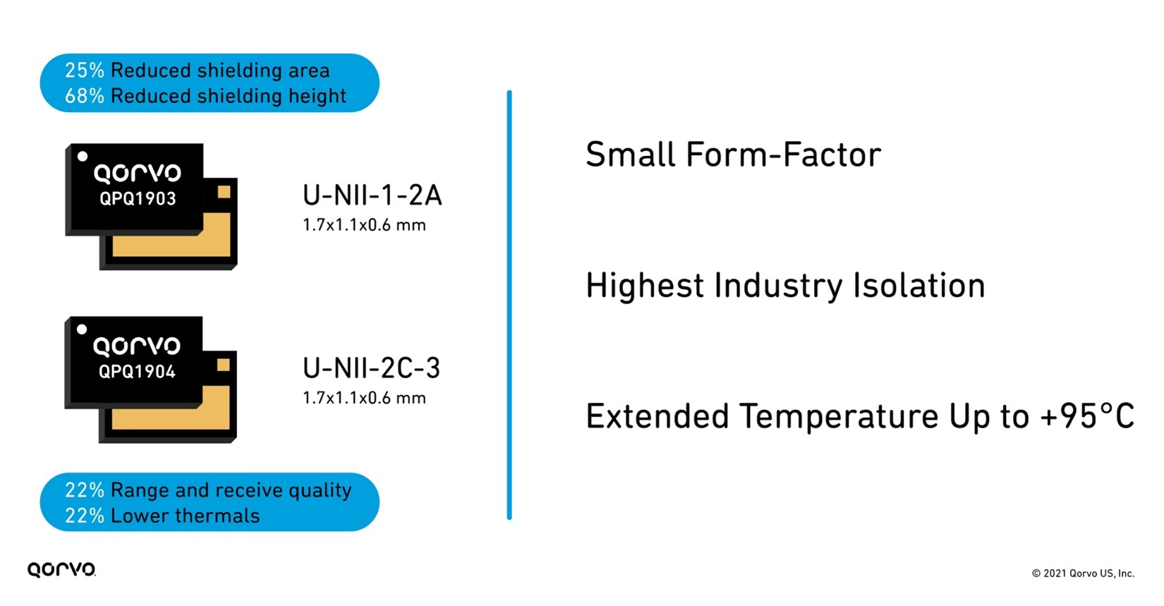
Figure 5: Benefits of using QPQ1903 and QPQ1904 bandBoost filters
The addition of multiple-input multiple-output (MIMO) and higher frequencies in the 6 GHz range increases system temperatures. With more thermal requirements, robust RFFE components are a must. Much of the industry specifies their parts in the 60°C to 80°C range, but higher temperature operation is needed based on the system temperatures produced in this frequency range. To solve these challenges, many hours of design effort have been spent on increasing the temperature capabilities of BAW. As product designs in Wi-Fi 5, 6/6E, and soon to come Wi-Fi 7, development has become more challenging, and as new opportunities like the automotive area opened for BAW, the push for higher temperature capability has come to the forefront.
Qorvo BAW technology engineers have delivered innovative devices by designing those that exceed the usual 85°C maximum temperature working range, going up to +95°C. The benefits this creates are great for both product designers and end-product customers. Now sleeker devices are achievable, as end-products no longer require large heat sinks. This also reduces design time as engineers can more easily attain system thermal requirements. One other advancement related to heat is that the bandBoost BAW products work at +95°C while still meeting a 0.5 to 1 dBm insertion loss.
This lower insertion loss improves Wi-Fi range and receive quality by up to 22 percent. Lower insertion loss also means improved thermal capability and performance as the RF signal seen at the RFFE Low Noise Amplifier (LNA) is improved. Below, Figure 6 shows the features and benefits of the QPQ1903 and QPQ1904 edgeBoost™ BAW filter.
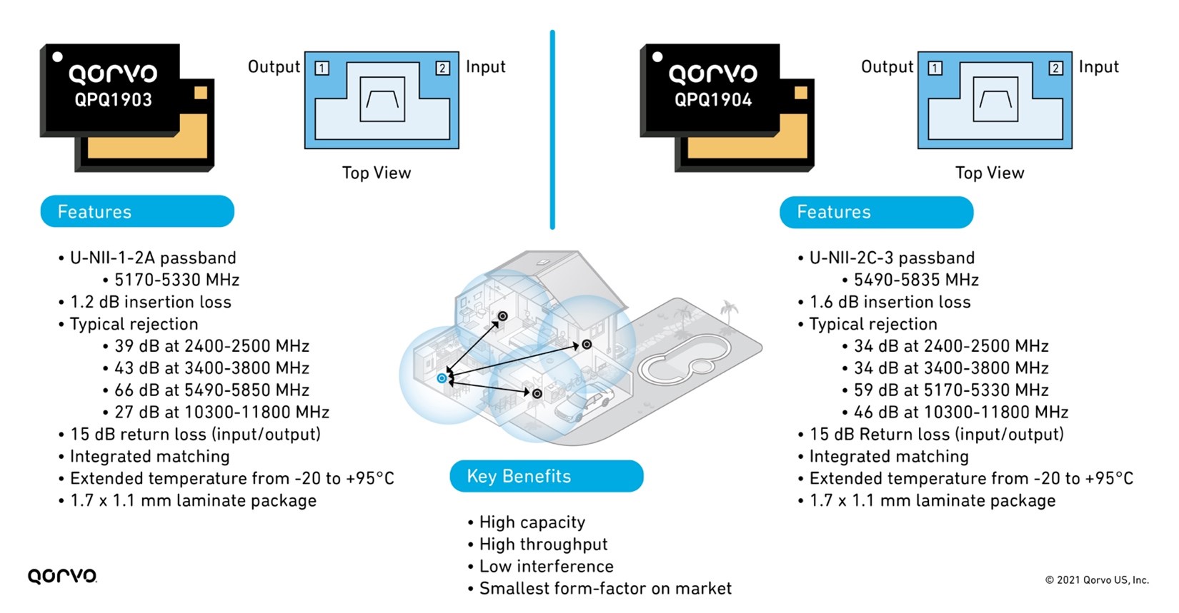
Figure 6: Features and benefits of QPQ1903 and QPQ1904
Not only are these filters providing benefits to the LNA, but they are small and perform well enough to install inside a tiny integrated Wi-Fi module package housing the LNA, switch, PA, and filter. Doing this drastically changes the end-product system layout making design easier and helps speed time-to-market. No longer are engineers burdened with matching and plugging individual passive and active components onto their PC board, but now they have all that done in these complex integrated modules called integrated front-end modules (iFEMs), creating a plug-and-play solution easily installed on their design.
A perfect example of this is the QPF7219 2.4 GHz iFEM, as seen in Figure 7. Qorvo has not only provided solutions with discrete edgeBoost BAW filters to increase output and capacity across all Wi-Fi channels. But Qorvo has gone a step further by including this filter inside an iFEM, our QPF7219, to provide customers with a drop-in pin-compatible replacement providing the same capacity and range performance outcome. This provides customers with design flexibility, board space in their design and is the first one of its kind on the market.
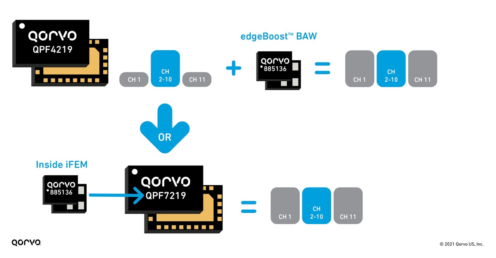
Figure 7: edgeBoost used as discrete and inside an iFEM
The need for smaller and sleeker product designs is always top of mind for Wi-Fi engineers. But to achieve the goal means component designers need to develop smaller products in many areas of the design, not just in one or two areas. From a tri-band Wi-Fi chip-set perspective, Qorvo has addressed this head-on. Qorvo has provided an entire group of iFEM alternatives to address the many signal transmit and receive lines in a product. This allows Wi-Fi design manufacturers to manage all the UNII and 2.4 GHz bands in a tri-band end-product design.
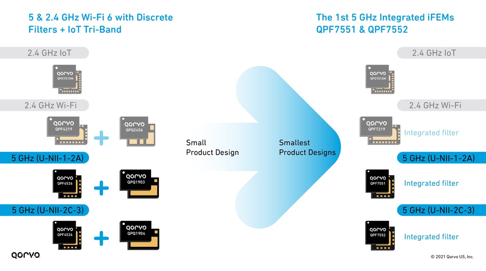
Figure 8: 2.4 & 5 GHz Wi-Fi 6 with IoT Tri-Band front-end solutions
This new design solution of combining the filter inside the iFEM equates to a smaller PC board and less shielding, as shown in Figure 9 below. Shielding matching and PC board space are expensive, not to mention the additional time associated with providing these materials. By placing all the RFFE materials inside a module, system designers can save cost, design faster, and get their products to market more quickly.
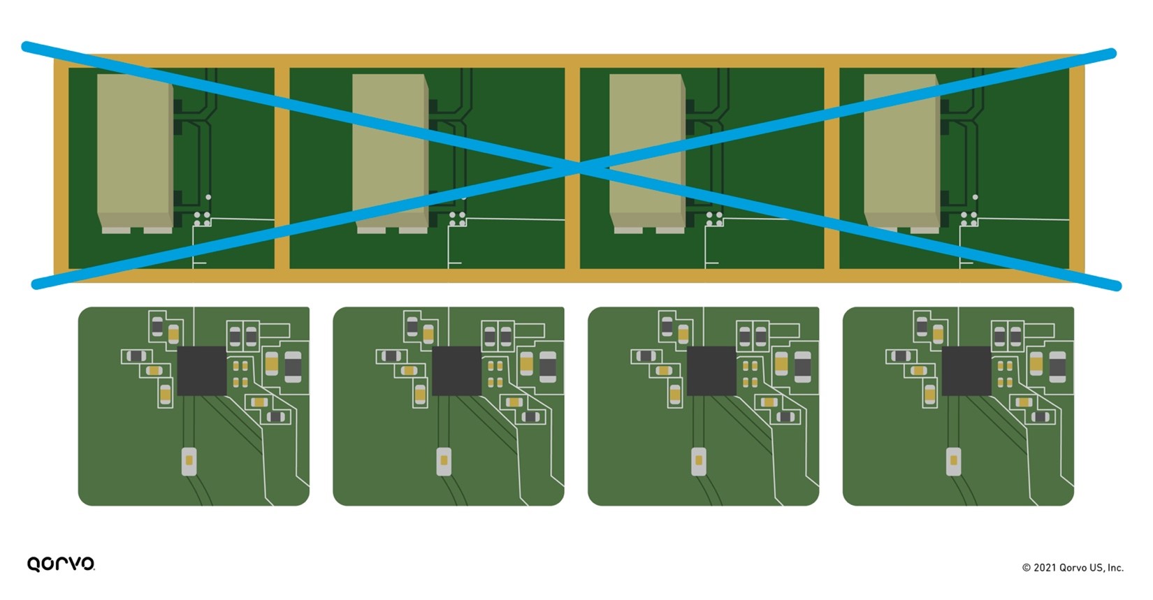
Figure 9: Putting the filter technology inside the iFEM removes shielding and reduces overall RFFE form-factor
As Wi-Fi system designers continue to be challenged with new specification requirements, they need newer or enhanced technologies to meet the need. By collaborating with our customers, we have provided state-of-the-art solutions to solve the tough thermal, performance, size, interference, capacity, throughput, and range difficulties seen by their end-customers. These solutions enable them to improve their designs to meet the Wi-Fi wave of today and in the future.