
As new CMIS standards are developed and adopted, with a wide variety of small form factor (SFF) and CMIS specs available, CMIS testing becomes increasingly complex and time consuming. The MultiLane Nexus Analyzer is a direct response to this complexity, designed with speed and simplicity at its core. A CMIS/SFF debug tool for interoperability testing and CMIS/SFF failures, the Nexus Analyzer is equipped with a full feature sweep implemented in its GUI.
Check out the below video from MultiLane, or read more.
Introduction
As a sales representative for ASUS, Starvoy is excited to announce the launch of the Tinker V, the first RISC-V single-board computer (SBC) from ASUS IoT. The Tinker V is designed for industrial IoT applications, with rich connectivity options, reliable technical support, and an open-source architecture. This powerful and versatile SBC is an excellent option for developers looking to build IoT solutions that are efficient, reliable, and built to last. If you’re looking for a powerful and dependable single-board computer for your next IoT project, Starvoy invites you to explore the possibilities of the Tinker V from ASUS. For further information please reach out to our sales team.

Open-Source Architecture
The Tinker V is equipped with a 64-bit RISC-V-based processor, which supports both Linux Debian and Yocto operating systems. This open-source architecture allows for flexibility in deployment and optimization, without incurring licensing and copyright fees.
Rich Connectivity Options
Designed to be compact, the Tinker V offers rich connectivity options and is specially engineered with a broad spread of peripheral connectors for industrial use, including GPIO, micro-USB, dual gigabit Ethernet, a pair of CAN bus interfaces, and two RS232 COM ports.
Built for Industrial IoT
The Tinker V is specially designed for industrial IoT applications, with an ultra-compact size, comprehensive functionality, and rich connectivity options. It also benefits from 1 GB of built-in RAM and an optional 16 GB eMMC, while supporting a wide range of operating temperatures from -20°C to 60°C.
Collaboration with Industry Leaders
ASUS IoT has collaborated with Renesas and Andes to accelerate the adoption of RISC-V and deployment in industrial IoT applications. The Tinker V SBC is specially designed to run Linux Debian and Yocto, making it the perfect choice for diverse IoT and gateway applications.
Conclusion
With its open-source architecture, broad connectivity options, and reliable technical support, the Tinker V is a versatile and reliable SBC for industrial IoT applications. If you are looking for a powerful and dependable single-board computer for your next IoT project, the Tinker V is an excellent option to consider.
For further information on the below, or other ams OSRAM products please reach out to the team.
Smart robots play an increasingly important role in industrial automation as well as in our homes. Smart robotics spans traditional robot arms in production lines (e.g. automotive manufacturers) to mobile robots used in logistics, so-called AGVs (automated guided vehicles), AMRs (autonomous mobile robots) in warehouses, or a robotic vacuum cleaner. ams OSRAM’s miniaturized sensing and illumination solutions. The better the robot understands and interacts with its dynamic environment, the more successful this technology becomes. Beside their unique portfolio of sensors, LEDs and lasers, ams OSRAM pursues a dedicated innovation roadmap regarding future technologies like smart-surface solutions and differentiating algorithms to advance robot capabilities.
Read More›In this industry, it can be easy to take power for granted. Easy, of course, until you don’t have it. Managing that vital resource is critical for systems to operate properly, and in a world that demands smaller, faster and smarter devices, it can be a real challenge. But what if a built-in power management device helped tackle that job? Qorvo’s Configurable Intelligent Power Solutions (ActiveCiPS™) devices help control, monitor and optimize power distribution and conversion in different systems with built-in intelligence and configurability.
In complex systems, or when a designer needs a more advanced or innovative power solution, it can be too expensive to use discrete components. Power Management Integrated Circuits (PMICs) integrate multiple voltage regulators and control circuits into a single chip. Today’s PMICs are flexible, allowing users to update default settings like output voltages, sequencing, fault thresholds and other parameters. As a result, PMICs are used in many small devices such as wearables, hearables and IoT (Internet of Things) devices – all thanks to their small size, high efficiency and low power consumption. These tiny, high-performance PMICs maximize system efficiency and performance while providing design flexibility and lowering the bill-of-materials cost.
Read More›
Blog post from partner: https://www.gsitechnology.com/
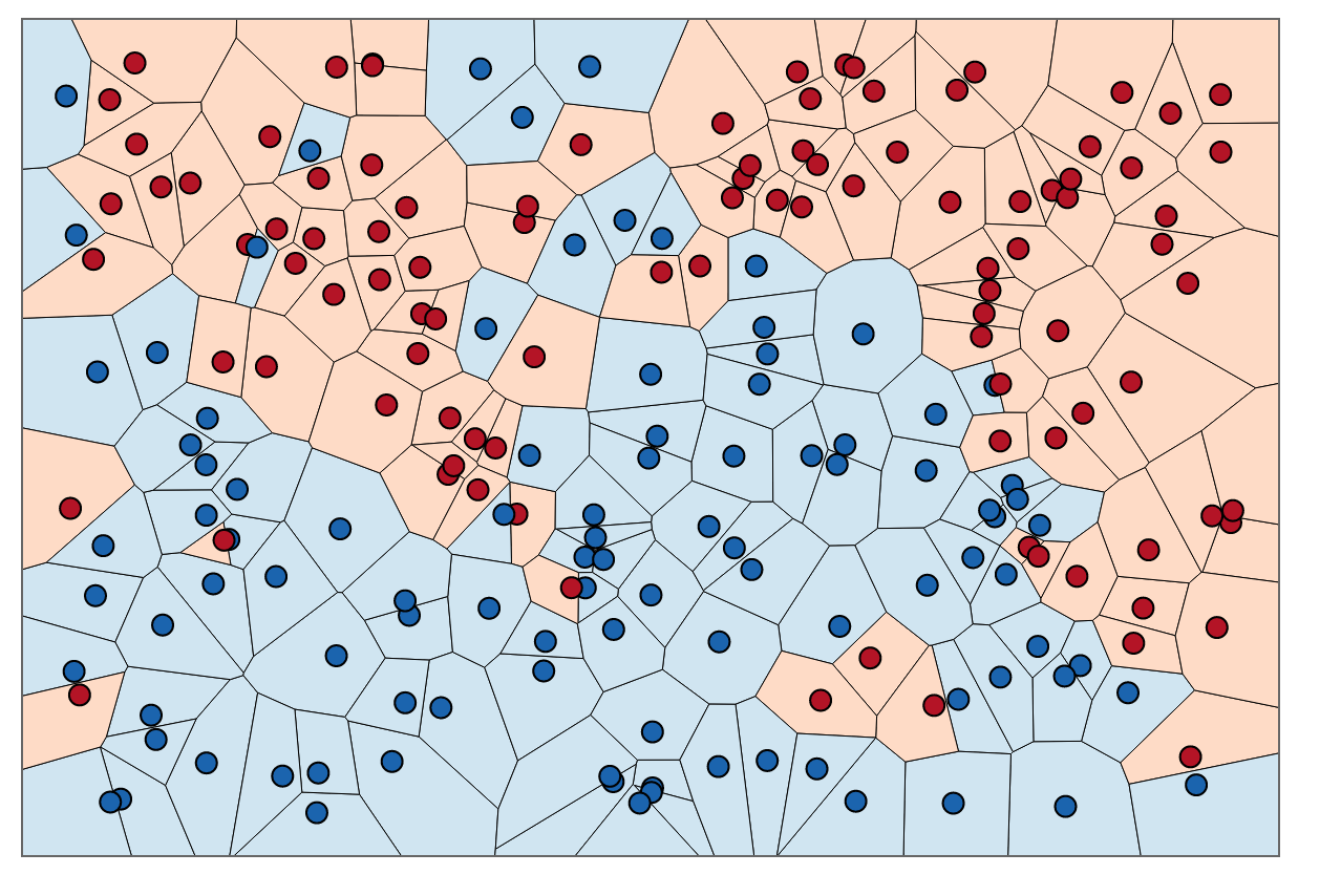
Approximate Nearest-Neighbors for new voter party affiliation. Credit: http://scott.fortmann-roe.com/docs/BiasVariance.html
Introduction
The field of data science is rapidly changing as new and exciting software and hardware breakthroughs are made every single day. Given the rapidly changing landscape, it is important to take the appropriate time to understand and investigate some of the underlying technology that has shaped and will shape, the data science world. As an undergraduate data scientist, I often wish more time was spent understanding the tools at our disposal, and when they should appropriately be used. One prime example is the variety of options to choose from when picking an implementation of a Nearest-Neighbor algorithm; a type of algorithm prevalent in pattern recognition. Whilst there are a range of different types of Nearest-Neighbor algorithms I specifically want to focus on Approximate Nearest Neighbor (ANN) and the overwhelming variety of implementations available in python.
My first project with my internship at GSI Technology explored the idea of benchmarking ANN algorithms to help understand how the choice of implementation can change depending on the type and size of the dataset. This task proved challenging yet rewarding, as to thoroughly benchmark a range of ANN algorithms we would have to use a variety of datasets and a lot of computation. This would all prove to provide some valuable results (as you will see further down) in addition to a few insights and clues as to which implementations and implementation strategies might become industry standard in the future.
What Is ANN?
Before we continue its important to lay out the foundations of what ANN is and why is it used. New students to the data science field might already be familiar with ANN’s brother, kNN (k-Nearest Neighbors) as it is a standard entry point in many early machine learning classes.
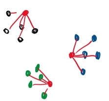
Red points are grouped with the five (K) closest points.
kNN works by classifying unclassified points based on “k” number of nearby points where distance is evaluated based on a range of different formulas such as Euclidean distance, Manhattan distance (Taxicab distance), Angular distance, and many more. ANN essentially functions as a faster classifier with a slight trade-off in accuracy, utilizing techniques such as locality sensitive hashing to better balance speed and precision. This trade-off becomes especially important with datasets in higher dimensions where algorithms like kNN can slow to a grueling pace.
Within the field of ANN algorithms, there are five different types of implementations with various advantages and disadvantages. For people unfamiliar with the field here is a quick crash course on each type of implementation:

- Brute Force; whilst not technically an ANN algorithm it provides the most intuitive solution and a baseline to evaluate all other models. It calculates the distance between all points in the datasets before sorting to find the nearest neighbor for each point. Incredibly inefficient.
- Hashing Based, sometimes referred to as LSH (locality sensitive hashing), involves a preprocessing stage where the data is filtered into a range of hash-tables in preparation for the querying process. Upon querying the algorithm iterates back over the hash-tables retrieving all points similarly hashed and then evaluates proximity to return a list of nearest neighbors.
- Graph-Based, which also includes tree-based implementations, starts from a group of “seeds” (randomly picked points from the dataset) and generates a series of graphs before traversing the graphs using best-first search. Through using a visited vertex parameter from each neighbor the implementation is able to narrow down the “true” nearest neighbor.
- Partition Based, similar to hashing, the implementation partitions the dataset into more and more identifiable subsets until eventually landing on the nearest neighbor.
- Hybrid, as the name suggests, is some form of a combination of the above implementations.
Because of the limitations of kNN such as dataset size and dimensionality, algorithms such as ANN become vital to solving classification problems with these kinds of constraints. Examples of these problems include feature extraction in computer vision, machine learning, and many more. Because of the prominence of ANN, and the range of applications for the technique, it is important to gauge how different implementations of ANN compare under different conditions. This process is called “Benchmarking”. Much like a traditional experiment we keep all variables constant besides the ANN algorithms, then compare outcomes to evaluate the performance of each implementation. Furthermore, we can take this experiment and repeat it for a variety of datasets to help understand how these algorithms perform depending on the type and size of the input datasets. The results can often be valuable in helping developers and researchers decide which implementations are ideal for their conditions, it also clues the creators of the algorithms into possible directions for improvement.
Open Source to the Rescue

Utilizing the power of online collaboration we are able to pool many great ideas into effective solutions
Beginning the benchmarking task can seem daunting at first given the scope and variability of the task. Luckily for us, we are able to utilize work already done in the field of benchmarking ANN algorithms. Aumüller, Bernhardsson, and Faithfull’s paper ANN-Benchmarks: A Benchmarking Tool for Approximate Nearest Neighbor Algorithms and corresponding GitHub repository provides an excellent starting point for the project.
Bernhardsson, who built the code with help from Aumüller and Faithfull, designed a python framework that downloads a selection of datasets with varying dimensionality (25 to nearly 28,000 dimensions) and size (few hundred megabytes to a few gigabytes). Then, using some of the most common ANN algorithms from libraries such as scikit-learn or the Non-Metric Space Library, they evaluated the relationship between queries-per-second and accuracy. Specifically, the accuracy was a measure of “recall”, which measures the ratio of the number of result points that are true nearest neighbors to the number of true nearest neighbors, or formulaically:
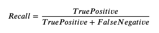
Intuitively recall is simply the correct predictions made by the algorithm, over the total number of correct predictions it could have made. So a recall of “1” means that the algorithm was correct in its predictions 100% of the time.
Using the project, which is available for replication and modification, I went about setting up the benchmark experiment. Given the range of different ANN implementations to test (24 to be exact), there are many packages that will need to be installed as well as a substantial amount of time required to build the docker environments. Assuming everything installs and builds as intended the environment should be ready for testing.
Results

After three days of run time for the GloVe-25-angular dataset, we finally achieved presentable results. Three days of runtime was quite substantial for this primary dataset, however as we soon learned this process can be sped up considerably. The implementation of the benchmark experiment defaults to running benchmarks twice and averaging the results to better account for system interruptions or other anomalies that might impact the results. If this isn’t an issue, computation time could be halved by only performing the benchmark tests once each. In our case we wanted to match Bernhardsson’s results so we computed the benchmark with the default setting of two runs per algorithm which produced the following:
Our results (top) and Bernhardsson’s results (bottom):

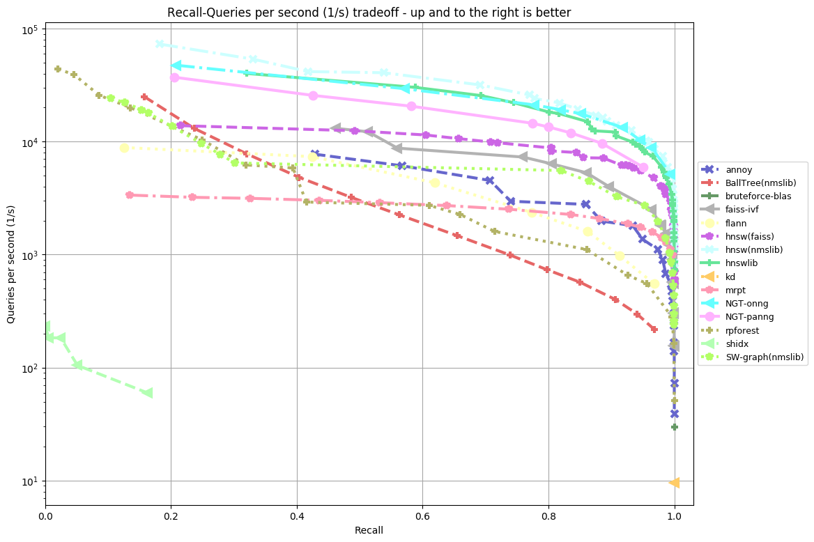
My Results vs Bernhardsson’s Results
As you can see from the two side by side plots of algorithm accuracy vs algorithm query speed there are some differences between my results and Bernhardsson’s. In our case, there are 18 functions plotted as opposed to 15 in the other. This is likely because the project has since been updated to include more functions following Bernhardsson’s initial tests. Furthermore, the benchmarking was performed on a different machine to Bernhardsson’s which likely produced some additional variability.
What we do see which is quite impressive is that many of the same algorithms that performed well for Bernhardsson also performed well in our tests. This suggests that across multiple benchmarks there are some clearly well-performing ANN implementations. NTG-onng, hnsw(nmslib) and hnswlib all performed exceedingly well in both cases. Hnsw(nmslib) and hnswlib both belong to the Hierarchical Navigable Small World family, an example of a graph-based implementation for ANN. In fact, many of the algorithms tested, graph-based implementations seemed to perform the best. NTG-onng is also an example of a graph-based implementation for ANN search. This suggests that graph-based implementations of ANN algorithms for this type of dataset perform better than other competitors.
In contrast to the well-performing graph-based implementations, we can see BallTree(nmslib) and rpforest both of which in comparison are quite underwhelming. BallTree and rpforest are examples of tree-based ANN algorithms (a more rudimentary form of a graph-based algorithm). BallTree specifically is a hybrid tree-partition algorithm combining the two methods for the ANN process. It is likely a series of reasons that cause these two ANN algorithms to perform poorly when compared to HNSW or NTG-onng. However, the main reason seems to be that tree-based implementations execute slower under the conditions of this dataset.
Although graph-based implementations outperform other competitors it is worth noting that graph-based implementations suffer from a long preprocessing phase. This phase is required to construct the data structures necessary for the computation of the dataset. Hence using graph-based implementations might not be ideal under conditions where the preprocessing stage would have to be repeated.
One advantage our benchmark experiment had over Bernhardsson’s is our tests were run on a more powerful machine. Our machine (see appendix for full specifications) utilized the power of 2 Intel Xeon Gold 5115’s, an extra 32 GBs of DDR4 RAM totaling 64 GBs, and 960 GBs of solid-state disk storage which differs from Bernhardsson’s. This difference likely cut down on computation time considerably, allowing for faster benchmarking.
A higher resolution copy of my results can be found in the appendix.
Conclusion and Future Work

Further benchmarking for larger deep learning datasets would be a great next step.
Overall, my first experience with benchmarking ANN algorithms has been an insightful and appreciated learning opportunity. As we discussed above there are some clear advantages to using NTG-onng and hnsw(nmslib) on low dimensional smaller datasets such as the glove-25-angular dataset included with Erik Bernhardsson’s project. These findings, whilst coming at an immense computational cost, are none the less useful for data scientists aiming to tailor their use of ANN algorithms to the dataset they are utilizing.
Whilst the glove-25-angular dataset was a great place to start I would like to explore how these algorithms perform on even larger datasets such as the notorious deep1b (deep one billion) dataset which includes one billion 96 dimension points in its base set. Deep1b is an incredibly large file that would highlight some of the limitations as well as the advantages of various ANN implementations and how they trade-off between query speed and accuracy. Thanks to the hardware provided by GSI Technology this experiment will be the topic of our next blog.
Appendix
- Computer specifications: 1U GPU Server 1 2 Intel CD8067303535601 Xeon® Gold 5115 2 3 Kingston KSM26RD8/16HAI 16GB 2666MHz DDR4 ECC Reg CL19 DIMM 2Rx8 Hynix A IDT 4 4 Intel SSDSC2KG960G801 S4610 960GB 2.5″ SSD.
- Full resolution view of my results:
Sources
- Aumüller, Martin, Erik Bernhardsson, and Alexander Faithfull. “ANN-benchmarks: A benchmarking tool for approximate nearest neighbor algorithms.” International Conference on Similarity Search and Applications. Springer, Cham, 2017.
- Liu, Ting, et al. “An investigation of practical approximate nearest neighbor algorithms.” Advances in neural information processing systems. 2005.
- Malkov, Yury, et al. “Approximate nearest neighbor algorithm based on navigable small-world graphs.” Information Systems 45 (2014): 61–68.
- Laarhoven, Thijs. “Graph-based time-space trade-offs for approximate near neighbors.” arXiv preprint arXiv:1712.03158 (2017).
